SPADE V3.0 - Spanning-tree Progression Analysis of Density-normalized Events
Background:
SPADE is an analytical tool for single-cell cytometry
data analysis and visualization. It views single-cell data as a high-dimensional point cloud and extracts the shape of the cloud. Details of the algorithm and example applications are described in:
SPADE was originally developed and implemented in MATLAB. The version that generated all figures in the above papers can be found at SPADE V1.0 and SPADE V2.0.
What's new:
On this webpage, we provide an updated version, SPADE V3.0. Compared to previous versions, this update provides
If you find any bugs or have any question about the user's manual below, please contact peng.qiu@bme.gatech.edu, or qiupeng81@gmail.com.
Updates and Mailing List:
SPADE is still being improved. If you would like to be informed on the updates, please join our Google group for SPADE updates, by following the link or by emailing me. I promise there won't be many emails.
License conditions:
The SPADE software is freely available for academic use. A patent for SPADE has been applied for on behalf of Stanford University. For license conditions, please contact the Office of Technology Licensing at Stanford (Kirsten Leute, kirsten.leute@stanford.edu).
Installation:
We provide source code of our implementation of SPADE which requires Matlab. In addition, we also provide pre-compiled standalone version that can be used in PC and Mac without Matlab. Last updated 2017-11-22.
1. Installation of source code if you have Matlab (7 or higher) on your computer, regardless of whether it is PC or Mac:
(1) Download the source code: SPADE3_source_code.zip
(2) Unzip the downloaded file, and add the directory containing the unzipped files into Matlab path.
(3) Type "SPADE" and press enter, the software will show up.
Note: the bulk part of SPADE3.0 is written in Matlab, and a few heavy-lifting calculations are written in C for faster speed. If you are using PC and the software does not run properly, please install Microsoft Windows SDK7.1. If you run into trouble installing windows SDK, here is a link that contains solutions that may work for you.
2. Installation of pre-compiled standalone version in a PC without Matlab:
(1) (Optinal) Install Microsoft Windows SDK7.1. If you run into trouble installing it, here is a link that contains solutions that may work for you.
(2) Download pre-compiled version: SPADE3 MyAppInstaller_web.exe for PC
(3) Double click the downloaded file to start the installation process of SPADE and Matlab Runtime. If you see a Windows Pop-up saying that running this installation may be unsafe, clicking "More info" and then "run anyway" will start the installation process.
(4) By default, SPADE will be installed to "C:\Program Files\SPADE\SPADE3_2017_11_22_win\application\SPADE3_2017_11_22_win.exe".
(5) Double click the above file will start the software.
3. Installation of pre-compiled standalone version in a Mac without Matlab:
(1) Download pre-compiled version: SPADE3 MyAppInstaller_web.app for Mac
(2) Unzip. Press control and click on the unzipped file/app. Click open to start the installation process of SPADE and Matlab Runtime.
(3) By default, SPADE will be installed to "/Applications/SPADE/SPADE3_2017_11_22_mac/", and Matlab Runtime will be installed to "/Applications/MATLAB/MATLAB_Compiler_Runtime/v85/".
(4) Open a terminal. Type "/Applications/SPADE/SPADE3_2017_11_22_mac/application/run_SPADE3_2017_11_22_mac.sh /Applications/MATLAB/MATLAB_Runtime/v85/" and press enter, the software will start.
Note: The command above contains two parts, separated by one space. The first part is the path where SPADE is installed, and the second part is the path where the Matlab_Runtime is installed. If the installation path on your computer is different from the example here, please make modifications accordingly.
Note: Starting SPADE from a terminal enables the software to output it's running status and progress to the terminal. The software can be started without using terminal, but it's not recommended because the running status and progress information will not be visible.
User Manual:
(1) Create a new folder, copy to this new folder all the FCS files you want to analyze together.
Note 1: For raw fcs data files generated by CyTOF, SPADE3 can handle them directly. If you would like to use FlowJo to perform some initial gating and export the gated data to SPADE, please use the latest version of FlowJo V10, and export in FCS3.0 format. Otherwise, the exported fcs file won't be opened correctly by SPADE3.
Note 2: Data in the FCS files should be after compensation. For example, an FCS file can contain uncompensated raw values and compensation matrix in the file header (most common). In that case, SPADE3 is able to read the compensation matrix embedded in the file header and apply it to obtain compensated data. Another is that the FCS file contains compensated data and no compensation matrix in its header. Here are two example files: SimulatedRawData.fcs and mouseBM.fcs, which are the data behind Figures 1 and 2 in Qiu et al, Nat Biotech, 2011. In the following, we will use these two FCS files to illustrate how to use SPADE3.
Note 3: For users to easily play with FCS files, we provide two functions in SPADE3 source code: "readfcs_v2.m" and "writefcs_v2.m". These two functions can be used to read data and compensation information out of FCS files, and also generate FCS files.
Note 4: Since different flow cytometors and softwares may save fcs files into slightly different format, it is difficult to guarantee that SPADE3 works well with all fcs files. Therefore, we provide a way to allow users to check whether SPADE3 "sees" the correct (compensated) data. During the computation of local densities in step (6) below, SPADE3 creates a folder named "check_loaded_data". The folder contains one tab-delimited txt file for each fcs file. Each txt file contains the data for the first 10 cells/events, and can be opened by excel, which show the data that SPADE3 sees. If you load a fcs file into FlowJo and export it into CSV format, you will be able to use excel to obtain the uncompensated and compensated data that FlowJo sees. A comparison between the txt from SPADE3 and csv from FlowJo will be able to confirm whether SPADE3 loads the data correctly. If yes, we are good to go. If not, send me a message and I may be able to help.
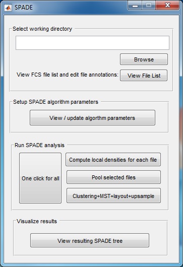
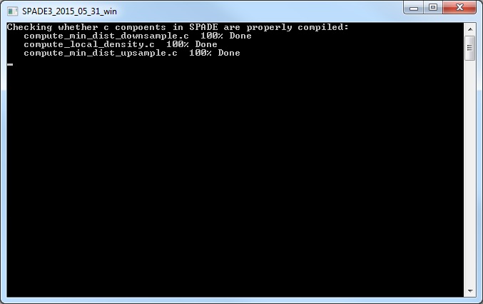
(2) Using the pre-compiled PC versions above, the main control window of the SPADE software will show up, as well as a windows command shell which displays the running status and progress of the program. If you have Matlab and use the source code version to start SPADE, the matlab command window displays software running status. If you use the pre-compiled version for Mac and start the software from a terminal, the software running status will be displayed in the terminal.
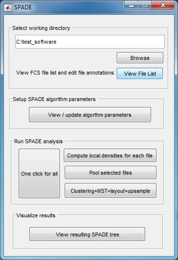
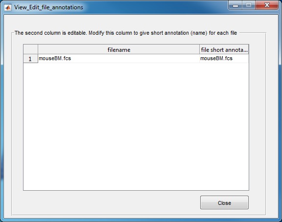
(3) Use the "Browse" button to select the directory that contains the FCS files to be analyzed. Another window will pop-up, which lists all FCS files in the selected folder. The second column is editable, in case the user wants to define a short name for each FCS file. Click the "close" button when finishing editing the second column. If you use the source code version in matlab, we recommend first changing the Matlab working directory to where the FCS files are stored and then start the SPADE software.
(4) Use the second panel of the main control window to setup algorithm parameters. The parameter setting will be stored in a file named "SPADE_paremeter.mat", in the same directory as the FCS files.
Important notes about parameter setting:
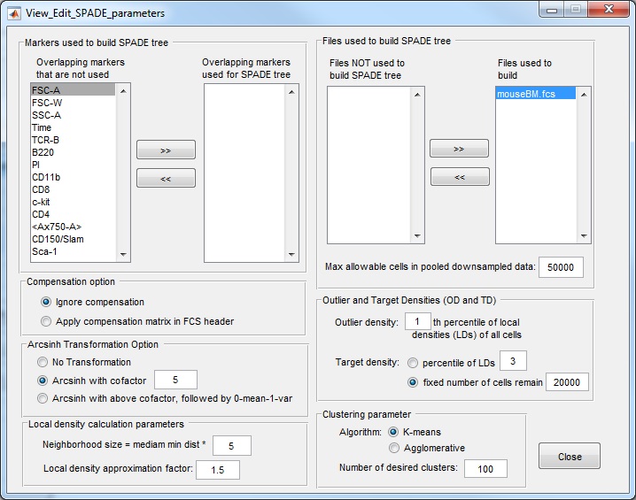
- When the parameter setting window is first opened, the upper-left corner contains a list of the overlapping markers that exist in all FCS files in the analysis folder. Users need to manually select markers that will be used to build the SPADE tree. If not, the software will give error in the subsequent steps.
- Which markers to use depends on what cell types/phenotype do we want to see in the SPADE tree. If we want the SPADE tree to represent cell types A, B and C, we need to include the protein markers that can define those cell types for SPADE tree construction, typically, the cell surface markers. Be sure to move markers to the list used for SPADE tree. Imagine you are performing manual gating on this dataset, what are the markers you would use during the manual gating process? Those are the markers that should be used to construct the SPADE tree.
- Compensation option: for fcs files from CyTOF, we should choose "ignore compensation", because there is no compensation needed and no compensation matrix stored in the file header. For fcs files from flow cytometry, if we choose the option of "apply compensation", SPADE will derive compensated data from the data and compensation matrix in the fcs file, so that the software operates on the compensated data. To check whether SPADE reads the data correctly, please refer to Note 4 under step (1) above.
- Transformation option: log-like transformations are often used to bring the data to log-scale. Here, we use the inverse hyperbolic sine transformation. For CyTOF data, we recommend the cofactor to be 5 (default value). For flow cytometry data, the cofactor can be 100, 150, or 200. I typically use 150. If the data stored in the fcs file is already after compensation and transformation, the software has the option to skip these two steps.
- Local density calculation for downsampling: although users are able to tune the values of the two parameters in the local density calculation (bottom left panel), we advise against changing those parameters. For all the flow and mass cytometry datasets we analyzed so far, we have been using the above default values.
- Outlier and target density parameters are the settings of downsampling one fcs file. The outlier density is the percentage of lowest density cells/events that are considered noise. The target density corresponds to the local density of cells that belong to the rare cell types that we want to capture. The above default setting means we consider 1% of cells with the lowest local density as noise and throw them away. Since it is difficult to know the local density of rare cell types a priori, we choose target density such that a fixed number of cells will survive the downsampling process, and the default value is 20000. If the total number of cells (after the 1% is thrown away) is smaller than 20000, no downsampling is performed.
- Max allowable cells parameter is useful when multiple fcs files are analyzed together. When multiple fcs files are processed together, if each results in 20000 cells after downsampling, the number of cells in the pooled downsampled data can be very large, and the subsequent clustering and upsampling steps can be very slow. To guard against that, we have a parameter "Max allowable cells in pooled downsampled data" whose default is 50000. If the pooled downsampled data has more cells than this parameter, we will perform further downsampling to reduce the number of cells to this parameter.
- Number of desired clusters . The key idea of SPADE is to over-cluster the data, so that the resulting tree is able to capture the underlying differentiation hierarchy among the cells. Therefore, we think there are 5 cell types in the data, we would want to ask for 50 or more clusters. The default number of clusters is 100, which is good when we use a small number of markers to build the tree. For CyTOF analysis where we want to distinguish more cell populations, we need to ask for more clusters, for example, 300.
- Deterministic downsampling to remove stochasticity. In the initial and earlier versions of SPADE, the downsampling step is stochastic, meaning that running the downsampling step on the same data twice will not give identical results, which further leads to differences in the subsequent clustering and tree construction steps. Although such randomness does not affect the statistics and interpretation of the final result, it creates unnecessary confusion. In this implementation, we developed a completely deterministic procedure for the downsampling steps, so that running the software twice on the same data will now give identical results. We are preparing a manuscript to describe details of this improvement.
- Example 1: SimulatedRawData.fcs (2-marker simulated CyTOF data, FCS3.0 format, no compensation), the appropriate setting is:
use both markers to construct the tree;
use cells in all files (only one here) to construct the tree;
ignore compensation;
use arcsinh and cofactor=5 to transform the data;
choose the outlier density 1%, and target densities such that 20000 will survive downsampling;
choose max allowable cells to be 50000;
choose the number of desired clusters to be 100;
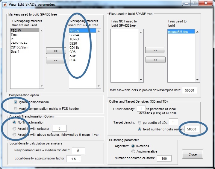
- Example 2: mouseBM.fcs (14-marker real mouse bone marrow flow cytometry data, FCS3.0 format, after compensation after transformation), the appropriate setting is:
use markers "FSC-A, SSC-A, TCR-B, B220, CD11b, CD8, c-kit, CD4" to construct the tree;
use cells in all files (only one here) to construct the tree;
ignore compensation;
no transformation;
choose the outlier density 1%, and target densities such that 50000 will survive downsampling;
choose max allowable cells to be 50000;
choose the number of desired clusters to be 100;
Here is a screenshot of the parameter setting for this mouseBM dataset:
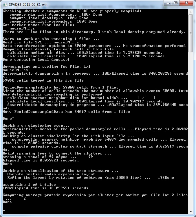
(5) After closing the parameter setting window, run SPADE by clicking the buttons in the third panel of the main control window. You can click the three small buttons sequentially (please wait until one button to finish before clicking the next one). Or, you can click the bigger button, which is equivalent to clicking the three smaller buttons sequentially. Since the downsampling step involves a lot of distance and density calculations, it can be slow. The windows command window (or matlab command window, or terminal) will display the running status and progress. Below is screenshot of the command window showing the SPADE software applied to the mouseBM.fcs data. We recommend running SPADE on a decent desktop or server, which can be faster than laptops. Note: SPADE will produce a number of .mat files to store intermediate results. One .mat file for each FCS file, plus two other .mat files.
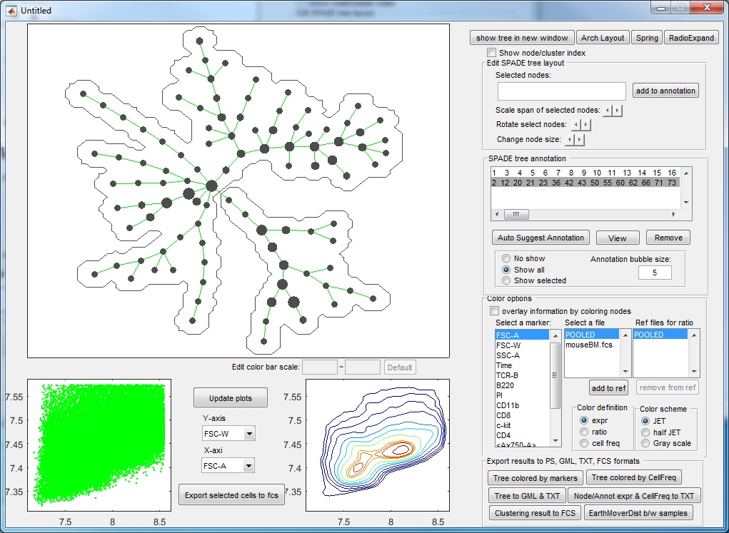
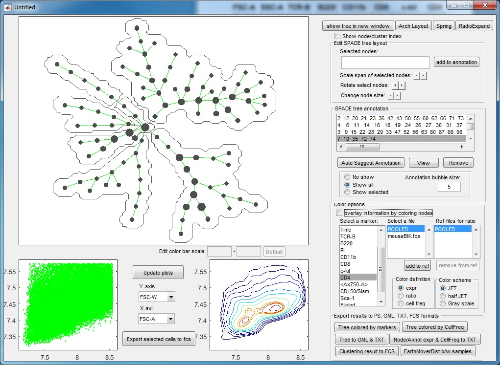
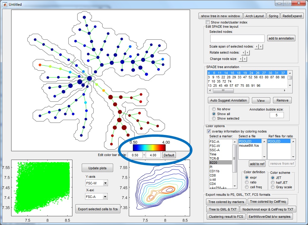
(6) Finally, to visualize the SPADE result, click the bottom button in the main control window. The following visualization window will show up. This figure is the SPADE result for mouseBM.fcs.
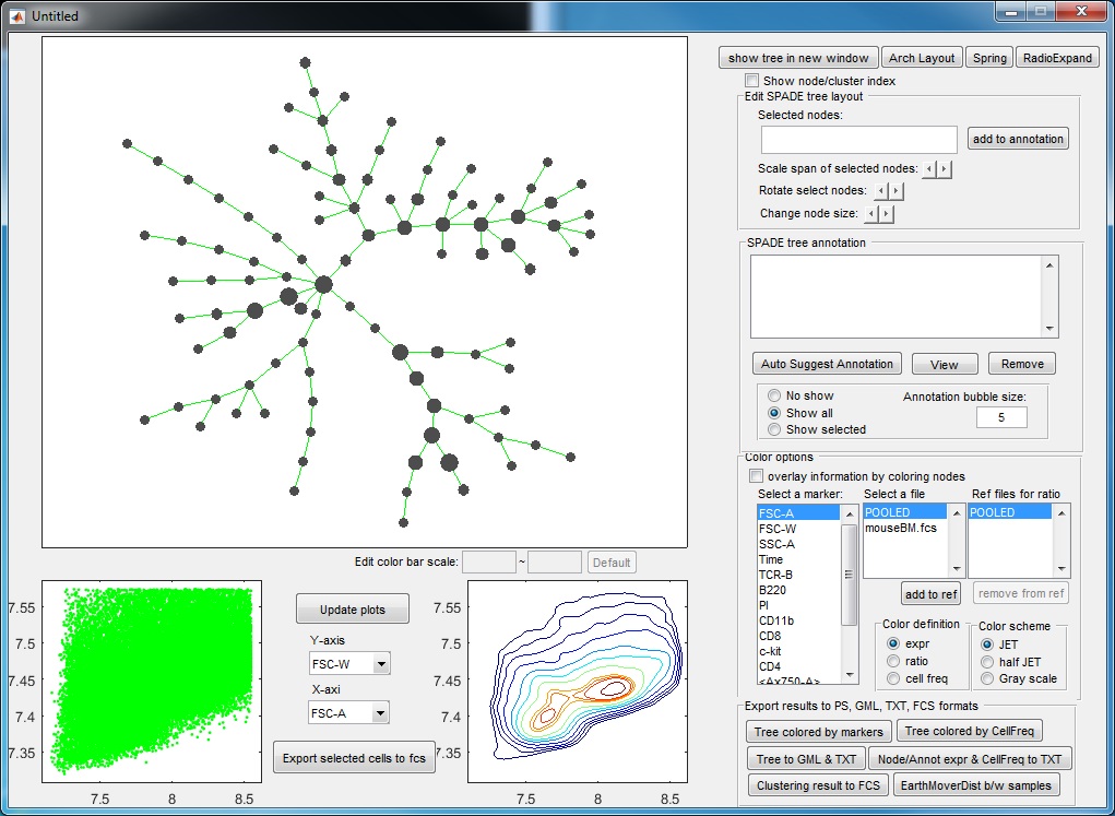
Meaning of the plots:
- The upper left panel shows the SPADE tree.
- The bottom panels are the dot plot and contour plot for the pooled downsampled cells. The axes are the values after compensation and transformation defined in the parameter setting window. Since these panels are based on downsampled data, in which the rare populations are enhenced, the contour plot here may look different from the contour plots drawn by FlowJo or other software.
Editing the tree:
- The tree nodes can be selected by mouse. The software also supports the use of
"Ctrl" and "Shift" keys together with the mouse. Numerical index of the selected
nodes are listed in the upper right editbox (next to the button named "add to
annotation"). The selection can be changed by
editing the content of that editbox.
- Selected nodes can be dragged around by mouse.
- Using the buttons in the edit SPADE tree panel, we can change the position of the selected nodes: rotate, expend and shrink.
- We can globally change the node size of all the tree nodes.
- By clicking the "Update plots" button in between the two bottom plots, cells in
the selected nodes will be overlaid on the biaxial plots.
- By clicking the "Export selected cells to fcs", a series of fcs
files will be generated, each containing the cells in selected nodes for one fcs file. This
function can be slow if the number of fcs files in this folder is large.
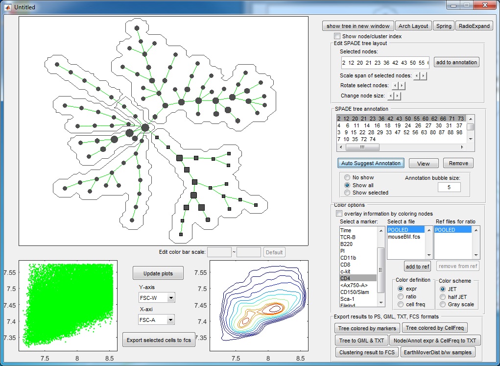
Semi-automated annotation of the tree:
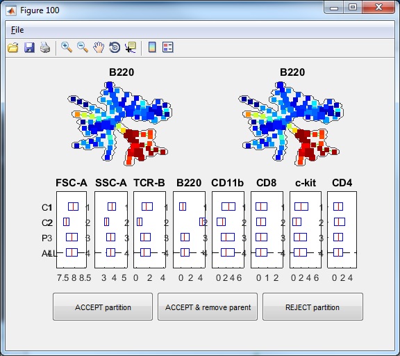
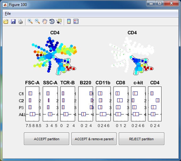
- Click the button "Auto Suggest Annotation", the software will examine the mouse-selected region of the tree (nodes shown in square not circles), or the entire tree if nothing is selected, and the software will automatically suggest the best edge to remove and break one piece of the tree into two pieces. One window will show-up showing the suggested partition. In this example dataset, if we click the "Auto Suggest Annotation", we will see the following figure. The software will look at the entire tree and suggest to remove one edge to break the tree into two pieces. This suggestion is based on all makers used to build the tree. From the boxplots, we can see that the two pieces ("C1" and "C2") differ by FSC-A, SSC-A, TCR-B and B220. "P3" indicate the combination of the two pieces and "ALL" represents the entire tree. In the top of the window, the SPADE tree is colored by the marker that shows the strongest difference between the two pieces, which is B220.
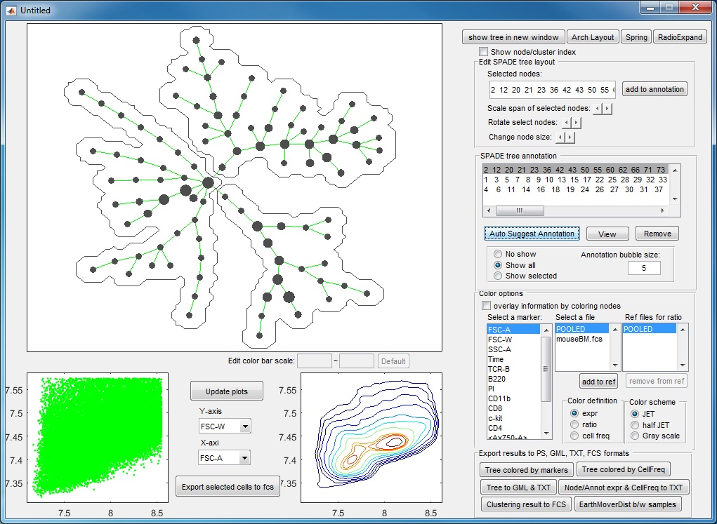
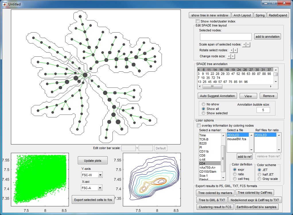
- If we click "ACCEPT & remove parent", the two pieces will be remembered, and the visualization window becomes the following.
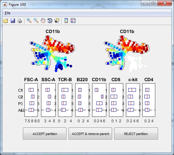
- If we click "Auto Suggest Annotation" again, the software will look at the entire tree and suggest the next edge to remove in the following figure. From the upper-right colored SPADE tree, we see that the second partition takes the bigger piece (colored region) from the first partition and breaks it into two smaller pieces according to CD11b expression. The boxplots confirm that.
- If we click "ACCEPT & remove parent", the annotation is remembered. Now, the tree is divided into three pieces of different phenotypes, and the visualization window becomes the following.
- After three more rounds of auto annotation, this SPADE tree is divided into 6 pieces, identifying major cell types in this dataset:
- At this point, if we click "Auto suggest annotation" again ,the software will split the upper right annotation into two pieces (dividing the CD11b+ cells into two subpopulation). Assume that we don't like to make this split, we can reject the suggested partition. When the auto suggested partitions are not good, we can manually guide the auto partition. For example, we can manually select a region of the tree by using the mouse to select or clicking the annotation listbox, the selected tree nodes will be shown as squares, and then we click "Auto Suggest Annotation". The software will only focus on the selected region of the tree and try to partition this region into two pieces, finding the best edge to remove within the manually selected region.
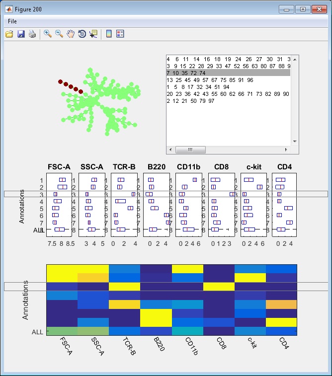
- Finally, we have the following annotations. If we click the "View" button, an interactive window will show up, summarizing the phenotypes of the annotations. One boxplot is draw for each marker, showing the distributions of the marker in different annotated tree regions, so that we can easily see which annotations are positive for this marker. The median values of all the boxplots are summarized into a heatmap representation. When we click the listbox and select one annotation, the correspond tree region will light up in the upper left figure. Therefore, this "View" provide two views of the partitioning results: (1) where are the clusters/annotations on the tree? (2) each partition are positive for what markers.
Manual annotation of the tree:
- If a set of nodes are selected and the user wants to draw a bubble around it to annotate this part of the tree, use the "add to annotation" to save the selection.
- The saved annotations are displayed in the listbox in the second panel of the right half of this window.
- The user can choose whether to display the annotations or not, using the three radiobuttons below the listbox for annotations.
Color the tree and interpretation:
- Select "expr" as color definition + select a marker used for tree construction + POOLED file: the tree shows how the selected protein marker behave across the entire tree. To compute the default numerical range of the colorbar, we compute the average marker expression in the tree nodes, and use the 5th and 95th percentiles to define the range. Typically, if the numerical range of the colorbar is comparable to the range of axis in the bottom panels (around of less than 5 fold difference), it means the cluster average of the marker is not drastically different from its expression in individual cells, and the color variation is interpretable. Otherwise, if the numerical range of the colorbar is too small (i.e. 20 time smaller than the range in the biaxial plot), the color variation is not interpretable, the select marker has little correlation with the other markers used to build the tree, and contribute little to the tree structure. Users are allowed to manually adjust the range of the colorbar.
- Select "expr" as color definition + select a marker used for tree construction + indivudial file: this selection does not make much sense, because the resulting colored tree will be extremely similar to the color when POOLED file is selected.
- Select "expr" as color definition + select a marker not used for tree construction + POOLED file, the tree again shows how the selected protein marker behave across the entire tree. If the selected marker is highly correlated to the ones used to build the tree (as if it can be included in defining the phenotypes), the numerical range of the colorbar will be comparable to the range of axis in the bottom panels (around of less than 5 fold difference), and the colored tree has the same interpretation as above. This typically works for protein markers whose behavior do not change across the fcs files. For proteins that behave differently across different fcs files (i.e., experimental conditions), we should not use POOLED file, it is better to use individual file, as in the next bullet.
- Select "expr" as color definition + select a marker not used for tree construction + indivudial file: this selection shows the behavior of one protein marker in a specific fcs file (experiment condition). It is helpful to compare the difference of the marker's behavior across conditions.
- Select "ratio" as color definition + select a marker not used for tree construction + indivudial file + another individual file for reference: this selection takes the behaviors of the selected marker in the two individual fcs files, and shows their difference. It is a subtraction in the transformed data. Since the arcsinh transformation is log-like, substraction in the transformed domain can be viewed as ratio in the original intensity scale.
- Select "ratio" as color definition + select a marker used for tree construction: this does not make sense, similar to the second point above.
- Selecting "cell freq" as color definition + an individual file is equivalent to selecting "expr" + "CellFreq" marker + individual file. This option colors the tree by the percentage of cells in each node for a selected file. This shows which parts of the tree are occupied by cells in the selected file.
- Selecting "ratio" as color definition + "CellFreq" marker + individual file + another individual file as ref. This option colors the tree by the percentage difference of cells in each node for the two selected files. It is equivalent to take two colored trees in the above bullet and display their difference in percentages.
- For the options "expr" and "ratio", if the color is defined based on an individual file and no cells in this file belong to a certain tree node, the node will be colored as white.
- In the file selection list and the reference file list, the software allows multiple files to be selected (ctrl or shift + mouse selection). In that case, node color will be defined based on average of the selected files, allowing visualization of average expr of multiple files (e.g. replica) and ratio between two groups of files.
Export results:
- Export tree figures colored by expression of each marker based on the pooled
data, into one single file "SPADE_tree_colored_by_markers.ps".
- Export tree figures colored by cell frequency computed based on each individual file,
into one single file "SPADE_tree_colored_by_CellFreq.ps".
- Export the topology and layout of the tree into GML and txt format, "SPADE_tree.gml",
"SPADE_tree_adjacency.txt" and "SPADE_tree_node_positions.txt".
- Export the average expression for each marker and each node/annotation ("SPADE_tree_node_annot_marker_expr.txt"),
counts of cells that belong to each node/annotation for each fcs file ("SPADE_tree_node_annot_cell_freq.txt"),
and definitions of the annotations ("SPADE_tree_annotation_definition.txt").
- Export the clustering results. For each fcs file, the software exports another
file, which contains an additional column that describes which node of the SPADE
tree each cell belongs to. This function might be slow if there are a large
number of fcs files in this analysis.
Note: upon closing this window,
edits of the tree layout and the annotations will be saved, so that the same
figures will show up next time is window is opened.
(7) When selecting the working directory from the main control window, if the selected directory is already analyzed, the user can directly view the results, by clicking the bottom button in the main window.
(8) There is a new button in the bottom right corner, related to uploading annotations to cytobank. This new functionality allows our SPADE implementation to interact with data and analysis on cytobank. More information about this new functionality will be provided later.