Sample Progression Discovery (SPD) version 1

Peng Qiu¹, Andrew Gentles², Sylvia Plevritis^2
1Department of Bioinformatics and Computational Biology, University of Texas MD Anderson Cancer Center
²Department of Radiology, Stanford University

We present a novel computational approach, Sample Progression Discovery (SPD), to discover patterns of biological progression underlying a microarray dataset. In contrast to the majority of microarray data analysis methods which focus on identifying differences between sample groups (i.e. normal vs. cancer, treated vs. control), SPD aims to identify an underlying progression among individual samples, both within and across sample groups. We applied SPD to gene expression data of cell cycle, B-cell differentiation, and mouse embryonic stem cell differentiation, where the underlying progression was known but hidden from SPD. We show that SPD correctly identified the progression among samples and the gene modules that are associated with the progression. We view SPD as a hypothesis generation tool, when applied to datasets where the progression is unclear. For example, when applied to a microarray dataset of cancer samples, SPD would assume that the cancer samples collected from individual patients represent different stages during an intrinsic progression underlying cancer development. The inferred relationship among the samples may therefore indicate a pathway or hierarchy of cancer progression, which serves as a hypothesis to be tested.

The algorithm is implemented in Matlab 7, with a Graphic User Interface on top of it, designed and written by Peng Qiu.

A manuscript of this work is available: Peng Qiu, Anderw Gentles and Sylvia Plevritis, "Discovering Biological Progression underlying Microarray Samples", PLoS Computational Biology, vol. 7, issue 4, e1001123, 2011.

This software is new and still being developed. Updates and new versions will available at here

If you have any questions or find any problems in it, please email me at peng.qiu@bme.gatech.edu 

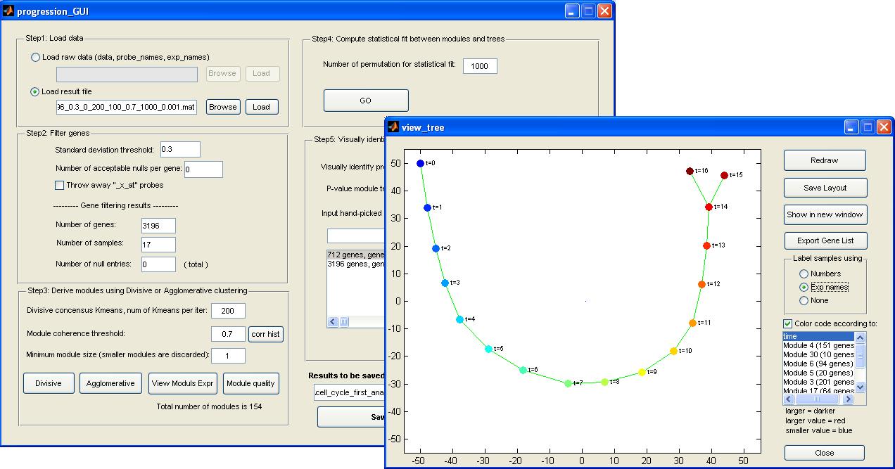
Here is a screen shot of our software

Installation instructions:

This package requires Matlab 7. In order to give users maximum freedom of manipulating this software, the raw .m files are provided.

    (1) download the zip package at: SPD.zip (last updated on April 28, 2011)

    (2) unzip to your local machine

    (3) open Matlab 7 and change the directory to where the package is unzipped, or add that directory to matlab path

    (4) type "progression_GUI" and enter, the GUI will show up


We also provide several example data and result files, which is available at
SPD_example_data_files.zip 

License conditions:

The SPD software is free for academic use. A patent for SPD has been applied for on behalf of Stanford University. For license conditions, please contact the Office of Technology Licensing at Stanford (Kirsten Leute, kirsten.leute@stanford.edu).

User Manual:

1. Prepare input file:

Input file contains at least 3 variables:
                probe_names : n * 1 cell array, each element is the name of one gene/feature
                exp_names : 1 * m cell array, each element is the name of one sample/array
                data : n * m expression data matrix

Two optional variables can be used to input clinical information or other sample annotations
                color_code_names: k * 1 cell array
                color_code_vectors: k * m matrix that stores clinical info

                For example:

                color_code_names = [ {'Gender'};
                                                        {'Tumor Grade'};
                                                      ];
                color_code_ vectors= [ 0 0 0 0 0 0 1 1 1 1 1 0 0 1 1;
                                                         1 2 3 2 2 2 1 1 3 3 3 2 1 1 1;
                                                       ];
       
An input file can contain other variables, but the software will just ignore them.

See examples at SPD_example_data_files.zip 



2. Load data

Users can load (1) a raw input data file defined above, or (2) a result file generated by the software.



3. Filter genes

Filter genes according to user-defined threshold of standard deviation, and number of acceptable nulls per gene. Any genes with smaller STD or more NULL entries are excluded. A user can also choose to exclude "_x_at" probesets.

The software shows some basic information after the filtering: number of genes left, number of samples, number of mull entries.

After filtering genes, null entries are imputed / filled using KNN imputation, so that the subsequent steps do not have to worry about null entries.

If more sophisticated filters are needed, users can apply those filters when preparing the input file, and then ignore the gene filtering functions in the GUI.



4. Clustering genes (Step 1 in SPD)

This software has two clustering algorithms, "Divisive" and "Agglomerative". My suggestion is always use "Agglomerative".

(1) Button "Divisive" launches the top-down consensus k-means clustering method that is described in the manuscript. Users can define the number of k-means iterations in each consensus k-means partitioning during the top-down process. Default is 200. Users can also define the stopping criterion, which is the desired module coherence. The default is 0.7, but this could be dataset-dependent. The button "corr hist" can be used to view a histogram of all the pair-wise correlation (after genes are filtered). If the histogram has a heavy tail, meaning many gene pairs share high correlation, higher coherence parameter might be more appropriate.

(2) Button "Agglomerative" is another clustering algorithm, which is agglomerative. This algorithm only needs one parameter, the module coherence. This algorithm goes bottom-up.

The parameter "Minimum module size" can be used to exclude small clusters.

After the clustering algorithm finishes, the two buttons "view modules Expr" and "Model quality" are enabled. You can use these two buttons to visualize the clustering results.

5. Construct MSTs and compare modules and MSTs (step 2 and step 3 in SPD)

The "GO" button does the following:

(1) Construction one MST based on each gene module

(2) Compute the p-values of the statistical concordance between all the modules and all the trees. Random permutation is performed to get the p-values. Users can define the number of random permutations, before clicking the GO button.

6. Identify modules similar in terms of progression (step 4 in SPD)

To generate a progression-similarity matrix between gene modules, users need to define a p-value threshold that determines whether the fit between a module and a tree is significant.

Then, click the button "Show gene module adjacency", a figure will pop up, which shows the similarity between modules, similarity in terms of progression.

Visually identify (high value) blocks along the diagonal. It is possible that there exist more than one block along the diagonal line.

Zoom-in this pop up window to see which modules are associated to the visually identified block(s).

Manually input the identified modules (a space-separated string that contains the IDs of the modules in the identified block) and click "add". After clicking "add", one entry will be shown in the list-box. This entry is one progression pattern defined by the modules that the user just "add"ed. (Multiple progression patterns can be added, each correspond to one block that the user visually identified).

To view the progression pattern, click "view progression". Another window will pop up. If the number of samples is smaller than 50, this step will take ~ 30 sec. If the number of samples is large, this step may take long, because my tree-visualization algorithm is slow.

In the pop-up window:
(1) Nodes/samples can be dragged around.
(2) After moving the nodes, the new layout can be saved. Then next time when the user views this progression pattern, the saved layout will be displayed, instead of running my slow tree-visualization algorithm. To save this new layout, you need to click the "Save Layout" button in the view_tree window, and the "Save Results" button in the main window.
(3) Nodes can be color-coded according to the modules that support this progression pattern (blue means low value, red means high value).
(4) Nodes can also be color-coded by the clinical information from the input data file: color_code_names, and color_code_vectors.
(5) Button "export gene list" writes two files in the current directory. Both contain the same information, the list of genes in the modules that support the progression.