Model reduction by MBAM (manifold boundary approximation method)
Here, we discuss model reduction using an example model for enzyme catalyzed reaction. We perform model reduction using the MBAM algorithm we previous developed (Transtrum & Qiu, PRL, 2014), and provide details and matlab code for the MBAM analysis. The basic idea of MBAM is to view the experimental data as a point in the data space and identify the nearest manifold boundary. The nearest boundary is identified by computing a geodesic path from a starting parameter estimated from the data, and travel along the canyons of the cost surface until a boundary/singularity is encountered. This boundary corresponds to a reduced model with one fewer degree of freedom, and it is able to better fit the data than reduced models corresponding to other boundaries of the manifold.
For detailed descriptions of the MBAM algorithm, code for the ODEgeodesics class used on this page, concept of model manifold and its relationship to experimental design, please visit the following link: publish_model_manifold.html.
Contents
Model for enzyme catalyzed reaction
Many biological reactions take the form of an enzyme catalyzed reaction in which an enzyme and a substrate combine reversibly to form an intermediate complex which can then disassociate as the enzyme and a product:  . These reactions can be modeled using the law of mass action as:
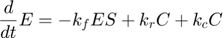
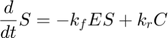

where  and
and  represent the reaction rates of the forward and reverse reaction of enzyme substrate association and dissociation.
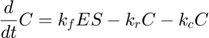
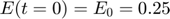
  represents the reaction rate of the enzyme-substrate complex converting to enzyme and product. Assume the initial condition of the system is:
Assume that the experimental data is measurement of the product at times  . Therefore, the mathematical description of the experiment is
 ![$[P(t=5), P(t=10), P(t=15)]$](publish_MBAM_example_eq04439191335428633218.png) .
.
MBAM - setting up the model
Here, we set up the model using a matlab-based geodesic integration tool. We assume the experimental data is [0.2589, 0.4898, 0.6712], which corresponds to to noise-free simulation of true underlying parameter value [1, 0, -1]. We would like to perform model reduction based on this observed data (true parameter) as starting point.
In the following, we first set up the model, including variables, parameters, equations, and initial conditions. The initial conditions are assumed to be constants, but they can also be parameters or functions of parameters.
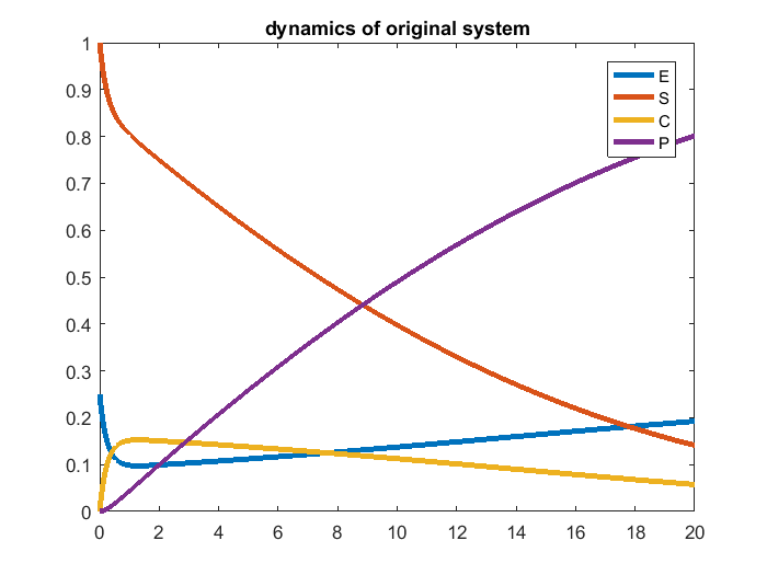
In addition, we simulate the system using the true parameter value, and visualize the simulation result.
% define name/symbol of the variables
x = [sym('E'); ...
     sym('S');...
     sym('C');...
     sym('P');...
     ];


% define name/symbol of parameters
theta = [sym('logkf'); ...
         sym('logkr');...
         sym('logkc');...
        ];


% define the right-hand-side of the ODE equations
dx = [-exp(theta(1)) * x(1) * x(2) + exp(theta(2)) * x(3) + exp(theta(3)) * x(3); ...
      -exp(theta(1)) * x(1) * x(2) + exp(theta(2)) * x(3); ...
       exp(theta(1)) * x(1) * x(2) - exp(theta(2)) * x(3) - exp(theta(3)) * x(3); ...
       exp(theta(3)) * x(3); ...
      ];


% define initial conditions of x
x0     = [sym('0.25');...
          sym('1');...
          sym('0');...
          sym('0');...
         ];

% dimension of the problem
M=length(x);        % number of dynamic variables
N=length(theta);    % number of parameters

% define observation configuration. Each row is one observation.
% First column indicates which variable observed.
% Second column is time point.
obs_config = [4, 5; ...
              4, 10; ...
              4, 15; ...
             ];   %In this eg, we observe P at time points 5, 10, 15


% construct an geodesic object of the ODEgeodesics class
obj = ODEgeodesics(x, dx, x0, theta, obs_config);

% compare the following three to the original system model:
disp('system dynamic variables:')
disp(obj.x)
disp('ODE right hand side:')
disp(obj.dx)
disp('initial conditions:')
disp(obj.x0)


% simulate the model with the above parameters
para = [1, 0, -1]';
time_points_to_plot = [0:0.01:20];
[t,y] = ode45(@(t,x_values)obj.ODE_rhs(t,x_values,para),[time_points_to_plot],obj.ODE_init(para));  % numerically integrate, evaluate at the observed time points. Important to add 0 as the first time point, because ODE45 views the first time point as the time of the initial condition
close all
figure(1)
plot(t,y(:,1:4),'linewidth',3); legend({'E','S','C','P'});xlim([min(t),max(t)]); title('dynamics of original system');
system dynamic variables:
 E
 S
 C
 P

ODE right hand side:
 C*exp(logkc) + C*exp(logkr) - E*S*exp(logkf)
                C*exp(logkr) - E*S*exp(logkf)
 E*S*exp(logkf) - C*exp(logkr) - C*exp(logkc)
                                 C*exp(logkc)

initial conditions:
 0.25
    1
    0
    0
MBAM - geodesics to find nearest manifold boundary
MBAM usually start from the observed experimental data and perform parameter estimation to obtain the starting point (starting parameter) for compute the geodesic path. In this example, since the experiment data corresponds to noise-free simulation of the true parameters, let's assume that the parameter estimation step is perfect, and start with the true parameter value for computing the geodesic path.
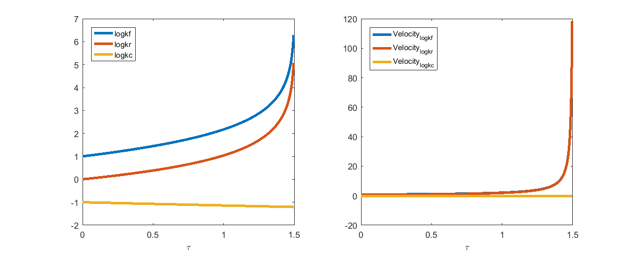
In the figure below, the left panel shows the computed geodesic path itself, and the right panel shows the velocity of the parameters along the path.
From both panels, we can see that the parameters and rapidly increase toward the end of the path. If we have infinite numerical precision and keep integrating along the geodesic path, and will eventually approach infinite. Another observation is that, along the path and especially toward the end, the difference between  and
and  approaches a constant, indicating that the ratio between the two parameters and approaches a constant. This limit can be used for deriving a reduced model.
% integrate and solve one geodesic path
obj = ODEgeodesics(x, dx, x0, theta, obs_config);                       % construct the object
obj = obj.compute_1st_order_sensitivity_equations;                      % compute 1st order sensitivity, needed for integrating geodesics
obj = obj.compute_2nd_order_sensitivity_equations;                      % only needed if we set obj.accerlation_compute_opt = '2nd_order_sensitivity_for_Gamma';
obj.integrate_method_opt = 'ODE_solver';                                % 'Euler' or 'ODE_solver' (preferred)
obj.accerlation_compute_opt = '2nd_order_sensitivity_for_Gamma';        % '2nd_order_finite_difference' or '2nd_order_sensitivity_for_Gamma'(preferred)
obj.smallest_singular_threshold = 1e-5;                                 % need some tuning for different models
obj.check_flipping_acceleration = 1;                                    % useful to guard against overshoot near symmetries
obj.display_integration_process = 1;
obj.para = [1, 0, -1]';                                                 % set initial parameter value. since the object is constructed using equations with log parameters, the numbers here are log values
[geodesic_path, tau] = obj.numerical_integrate_for_geodesic_path;       % integrate the geodesic path

% visualize result
h = figure(2); set(h, 'position', [100 100 1000 400])
subplot(1,2,1); plot(tau, geodesic_path(:,1:obj.N),'linewidth',3); xlabel('\tau'); legend(obj.display_parameter_names, 'Location', 'northwest')
subplot(1,2,2); plot(tau, geodesic_path(:,obj.N+1:end),'linewidth',3); xlabel('\tau'); legend(strcat('Velocity_{', obj.display_parameter_names, '}'), 'Location', 'northwest')
drawnow
current tau: 0 - current smallest singular value: 0.0016405
current tau: 0.001 - current smallest singular value: 0.0016396
current tau: 0.002 - current smallest singular value: 0.0016387
current tau: 0.003 - current smallest singular value: 0.0016377
current tau: 0.010892 - current smallest singular value: 0.0016304
current tau: 0.018785 - current smallest singular value: 0.001623
current tau: 0.026677 - current smallest singular value: 0.0016155
current tau: 0.03457 - current smallest singular value: 0.001608
current tau: 0.080771 - current smallest singular value: 0.0015646
current tau: 0.12697 - current smallest singular value: 0.0015202
current tau: 0.17317 - current smallest singular value: 0.0014744
current tau: 0.21937 - current smallest singular value: 0.0014309
current tau: 0.33539 - current smallest singular value: 0.0013131
current tau: 0.45141 - current smallest singular value: 0.001192
current tau: 0.56743 - current smallest singular value: 0.001069
current tau: 0.68345 - current smallest singular value: 0.00094248
current tau: 0.79947 - current smallest singular value: 0.00081396
current tau: 0.9159 - current smallest singular value: 0.00068262
current tau: 1.0032 - current smallest singular value: 0.0005834
current tau: 1.0757 - current smallest singular value: 0.00050035
current tau: 1.1482 - current smallest singular value: 0.00041653
current tau: 1.201 - current smallest singular value: 0.00035537
current tau: 1.2538 - current smallest singular value: 0.00029375
current tau: 1.2911 - current smallest singular value: 0.00025045
current tau: 1.3222 - current smallest singular value: 0.00021405
current tau: 1.3532 - current smallest singular value: 0.00017772
current tau: 1.3757 - current smallest singular value: 0.00015144
current tau: 1.3982 - current smallest singular value: 0.0001249
current tau: 1.4141 - current smallest singular value: 0.00010614
current tau: 1.4272 - current smallest singular value: 9.0758e-05
current tau: 1.4404 - current smallest singular value: 7.5096e-05
current tau: 1.4499 - current smallest singular value: 6.4073e-05
current tau: 1.4578 - current smallest singular value: 5.4956e-05
current tau: 1.4657 - current smallest singular value: 4.5619e-05
current tau: 1.4714 - current smallest singular value: 3.8838e-05
current tau: 1.4762 - current smallest singular value: 3.3234e-05
current tau: 1.481 - current smallest singular value: 2.7563e-05
current tau: 1.4844 - current smallest singular value: 2.351e-05
current tau: 1.4879 - current smallest singular value: 1.9395e-05
current tau: 1.4903 - current smallest singular value: 1.6564e-05
current tau: 1.4928 - current smallest singular value: 1.3686e-05
current tau: 1.4945 - current smallest singular value: 1.1606e-05
current tau: 1.4959 - current smallest singular value: 9.9209e-06
may need to stop, FIM singular
current tau: 1.4952 - current smallest singular value: 1.076e-05
current tau: 1.4956 - current smallest singular value: 1.0315e-05
current tau: 1.4958 - current smallest singular value: 1.014e-05
current tau: 1.4958 - current smallest singular value: 1.0025e-05
current tau: 1.4959 - current smallest singular value: 9.962e-06
may need to stop, FIM singular
current tau: 1.4959 - current smallest singular value: 9.9764e-06
may need to stop, FIM singular
current tau: 1.4959 - current smallest singular value: 1.0003e-05
current tau: 1.4959 - current smallest singular value: 1.0004e-05
current tau: 1.4959 - current smallest singular value: 1.0002e-05
current tau: 1.4959 - current smallest singular value: 9.9899e-06
may need to stop, FIM singular
current tau: 1.4959 - current smallest singular value: 9.9969e-06
may need to stop, FIM singular
current tau: 1.4959 - current smallest singular value: 9.9998e-06
may need to stop, FIM singular
current tau: 1.4959 - current smallest singular value: 1.0001e-05
current tau: 1.4959 - current smallest singular value: 1e-05
current tau: 1.4959 - current smallest singular value: 1e-05
current tau: 1.4959 - current smallest singular value: 1e-05
may need to stop, FIM singular
current tau: 1.4959 - current smallest singular value: 1e-05
current tau: 1.4959 - current smallest singular value: 1e-05
current tau: 1.4959 - current smallest singular value: 1e-05
may need to stop, FIM singular
current tau: 1.4959 - current smallest singular value: 1e-05
current tau: 1.4959 - current smallest singular value: 1e-05
current tau: 1.4959 - current smallest singular value: 1e-05
may need to stop, FIM singular
current tau: 1.4959 - current smallest singular value: 1e-05
current tau: 1.4959 - current smallest singular value: 1e-05
current tau: 1.4959 - current smallest singular value: 1e-05
current tau: 1.4959 - current smallest singular value: 1e-05
current tau: 1.4959 - current smallest singular value: 1e-05
may need to stop, FIM singular
current tau: 1.4959 - current smallest singular value: 1e-05
may need to stop, FIM singular
current tau: 1.4959 - current smallest singular value: 1e-05
may need to stop, FIM singular
current tau: 1.4959 - current smallest singular value: 1e-05
current tau: 1.4959 - current smallest singular value: 1e-05
may need to stop, FIM singular
current tau: 1.4959 - current smallest singular value: 1e-05
current tau: 1.4959 - current smallest singular value: 1e-05
current tau: 1.4959 - current smallest singular value: 1e-05
current tau: 1.4959 - current smallest singular value: 1e-05
current tau: 1.4959 - current smallest singular value: 1e-05
MBAM - the computed path travels along canyon of cost surface
MBAM algorithm aims to identify the geodesic path that travels along canyons of the cost surface, which leads to singularities while incurring minimum amount of changes in the model prediction, or in other words, minimum amount of increase in the cost function value.
Let's spell it out a little bit more. Since the starting point is obtained by parameter estimation that minimizes the least-square cost function, the cost function value at the starting point is at least a local minimum, and hopefully the global minimum. If we move the parameter away from the starting point and move along the geodesic path by MBAM, the cost is going to increase. If we move the parameter from the starting point along some other direction/trajectory, the cost is also going to increase. Since geodesic path by MBAM travels along canyons of the cost surface, it is the path that incur the smallest amount of increase in the cost function.
Since the model manifold of this example is bounded, if we move the parameter far enough (to either infinite or some symmetry), the image of the parameter in the data space on the manifold will for sure approach one manifold boundary, manifested by singularity in the Fisher Information Matrix and Jacobian Matrix. The geodesic path MBAM computes is the path that reaches the nearest boundary, and the path that reaches the boundary with minimum amount of increase in the cost function.
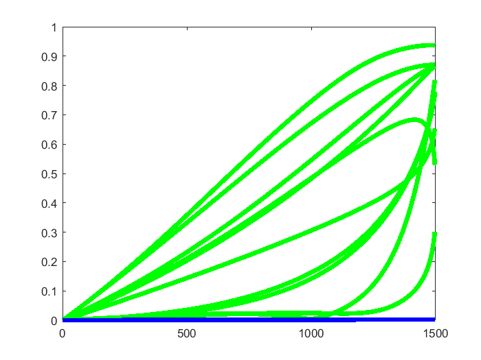
To visualize this, we created 10 randomly rotated version of the geodesic path MBAM computed, using the starting point as the origin for the rotation operation. For both the MBAM geodesic path and the randomly rotated paths, we computed the model prediction along those paths, and computed the difference between model predictions along the paths and the model prediction at the common starting point. This difference indicates the increase of the cost function incurred by moving along these paths. In the figure below, the blue curve shows the increase of cost along the MBAM path, which is very small in the order of 1e-3 and thus appears to be flat. The 10 green curves show the increase of cost along the 10 randomly rotated version, which are all larger. We see similar patterns when we generated more such randomly rotated paths. This provide some support that the MBAM path travels along the canyons.
computed_geodesic_path = geodesic_path(:,1:3);
model_prediction_at_starting_point = obj.compute_model_prediction(computed_geodesic_path(1,1:3)');
distortion_along_computed_path = zeros(size(computed_geodesic_path,1),1);
for i=1:size(computed_geodesic_path,1)
    distortion_along_computed_path(i) = norm(obj.compute_model_prediction(computed_geodesic_path(i,1:3)') - model_prediction_at_starting_point);
end

distortion_along_rotated_path = zeros(size(computed_geodesic_path,1),10);
for j=1:10
    rotated_geodesic_path = (rotx(rand*360)*roty(rand*360)*rotz(rand*360)*((computed_geodesic_path - computed_geodesic_path(1,:))'))' + computed_geodesic_path(1,:);
    for i=1:size(rotated_geodesic_path,1)
        distortion_along_rotated_path(i,j) = norm(obj.compute_model_prediction(rotated_geodesic_path(i,1:3)') - model_prediction_at_starting_point);
    end
end

figure(3)
plot(1:size(distortion_along_rotated_path,1), distortion_along_rotated_path,'g-',1:size(distortion_along_computed_path,1), distortion_along_computed_path,'b-','linewidth',4)
MBAM - derive reduced model using the limit suggested by the geodesic path
According to the MBAM geodesic path above, the limit we wish to evaluate is  . This limit leads to an equilibrium approximation which is the well-known Michaelis-Menten approximatiion. In one of our previous publications (Transtrum & Qiu, PLoS Comp Bio, 2016), we provided details of how to derive a reduced model based on this limit. Here we briefly repeat it.
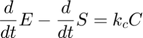
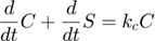
Since and always appear in the combination  , which participates in three of the four equations. We can isolate this motif by adding and subtracting
  to
to  and
and  respectively, giving:
Dividing the second above by , we have
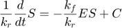
which becomes the following when the two parameters go to infinity while their ratio remains finite,
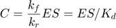
where we introduce  to represent the ratio of
  .
.
Furthermore, due to the conservation of the enzyme,  . Combining this relationship with the equation above, we have the following relationship:

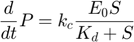
therefore, plugging  into the $dP/dt4 equation, we arrive at the Michaelis-Menten approximation:
The entire system can then be described by the following set of three differential equations plus one algebraic equation:
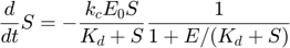
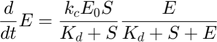
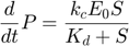
Overall, evaluating the MBAM-identified limit in this example removed one parameter, and along the process removed one dynamical variable.