Experimental Design and Model Reduction in Systems Biology
Mathematical modeling is undoubtedly an important tool for understanding complex biological systems, and for making predictions about system behavior far away from its nominal operating conditions. These models can take the form of ordinary differential equations (ODE), stochastic differential equations, Boolean networks, Bayesian networks, and other frameworks. In the case of ODE-based modeling, ordinary differential equations are often constructed by including prior knowledge of interactions among individual genes and proteins in the system. The models are often highly complex and contain many unknown parameters, such as reaction rates, binding affinity, and Hill coefficient. Compared to the complexity of the models, the amount of experimental data is almost always limited and not enough to constrain the parameters. As a result, it is possible that drastically different sets of parameters can fit the data equally well, which is a manifestation of an information gap between the model complexity and the data. Parameter estimation in this situation is an ill-posed problem, and thus very challenging.
To address this challenge, one strategy is to: develop better optimization algorithms for parameter estimation, and investigate sensitivity and identifiability to evaluate which parameters are accurately estimated and which ones have large uncertainty. Literature along this line is voluminous, and most progress took place in the fields of statistics, machine learning, systems and control theory. An alternative strategy is to make the problem better conditioned by obtaining more data or simplifying the model, with methods that are referred to as experimental design and model reduction in the literature. In this document, we will focus on the second strategy and present a few methods for experimental design and model reduction using a toy example.
Before going through the example and code below, readers need to go to the last section and download necessary functions supporting the examples shown on this page.
Contents
- Toy example: sum of two exponentials
- Experimental design problem setup
- Experimental design algorithm based on uncertainty quantification
- Experimental design algorithm based on profile likelihood
- Geometric interpretation of experimental design
- Model reduction problem setup
- Model reduction algorithm based on manifold boundaries
- Model reduction algorithm based on profile likelihood
- Remarks on the two model reduction algorithms
- A slightly larger example for model reduction
- Necessary functions
Toy example: sum of two exponentials
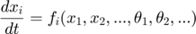
To introduce methods for experimental design and model reduction problem, we start with a simple toy example – the sum of two exponentials. Assume we have a black box containing two radioactive materials with different decay rates, and we would like to determine the values of the decay rates. From outside the box, we can only measure the total radiation level. For ease of discussion, we assume that at time t=0, the radiation levels of the two materials are both 1. This system can be modeled by the following ODEs.

where  and
and  represent the radiation levels of the two materials, which exponentially decay at rates
  and
and  .
.  is the total radiation we can measure. The simplifying assumption is modeled by the initial condition
  . Since this ODE system is linear, we can obtain its analytical solution below. However, this is special to this toy problem. For more complex systems biology models, such an explicit analytical solution is typically not available. The structure of the solution for is why we call this model the sum of two exponentials.


To determine the decay rates, we design an initial experiment, where we measure the total radiation level at time points t=1 and t=3. Thus, as the mathematical description of the experimental data:  is
is  , and
, and  is
is  .
.
A very important note here: a complete desciption of the model should include both mathematical descriptions of the system and mathematical descriptions of the experimental data.
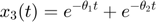
Using this toy example, we would like to introduce a few terminologies bolded in this paragraph. Since the systems has two unknown parameters, and , the parameter space is 2-dimensional. A 45 degree line is drawn in the parameter space because of the symmetry in the model. The experiment makes two measurements, and , and therefore the data space is 2-dimensional. The model (mathematical descriptions of both the system and the data together) defines a mapping from the parameter space to the data space. If we consider all parameter settings in the parameter space and map them to the data space, we will obtain a collection of points in the data space that are achievable by the model (shaded area in the figure below), which is what we call model manifold. Typically, the model manifold will not occupy the entire data space, because of the constraints/structure of the model
close all
h = figure(1); set(h,'position',[100   100   1000   450])
subplot(1,5,1:2);
patch([0 20 20 0 0],[0 0 20 20 0],[0.7,0.7,0.7])
axis([0 20 0 20])
hold on; plot([0 20], [0,20], '--k'); hold off
title('Parameter space','Fontsize',15)
xlabel('\theta_1','Fontsize',12)
ylabel('\theta_2','Fontsize',12)
subplot(1,5,4:5);
theta=20:-0.01:0;
y1 = [exp(-theta*1), 1+exp(-theta*1), fliplr(2*exp(-theta*1))];
y2 = [exp(-theta*3), 1+exp(-theta*3), fliplr(2*exp(-theta*3))];
patch(y1,y2,[0.7,0.7,0.7])
axis([-0.5 2.5 -0.5 2.5])
title('Data space','Fontsize',15)
xlabel('obs_1','Fontsize',12)
ylabel('obs_2','Fontsize',12)
drawnow
snapnow
Experimental design problem setup
Experimental design is needed when we deal with an information gap between a highly complex ODE model in systems biology and a limited amount of experimental data. In this case, one intuitive approach to bridge the gap is to obtain more data by performing new experiments. To design a new experiment, we typically need to decide what perturbation (activation or inhibition) is to be applied to which components (genes and proteins) of the system, as well as which components should be measured at which time points. These choices together constitute the design of a new experiment. Overall, the experimental design question we want to answer is: given an ODE model and limited experimental data, if we are allowed to perform one additional experiment, what experiment is maximally informative in improving parameter estimation?
Albeit the simplicity of the toy example model above, it represents a nonlinear relationship between the parameter space and the model manifold. Therefore, we can create a situation where measuring at the two time points ( and
and  ) does not provide enough information to estimate the model parameters.
Assume we have performed the experiment and the observed data are  and
and  (corresponding to noise-free observation of true underlying parameter
  ). Of course, assume we do not know the underlying parameter values, and we would like to estimate them using the observed data.
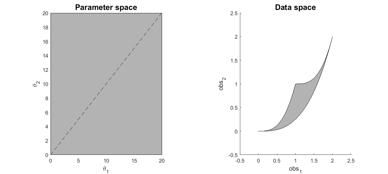
This is, in fact, a situation where the data does not contain enough information compared to the complexity of the model. There are two ways to explain this. (1) The measured variable is a sum of exponential decays that will eventually go down to 0. By the time that the two measurements are taken, is already extremely close to 0. Because the measurements are taken too late, there is little information in the observed data to figure out the model parameters. (2) The data corresponds to one point (star) in the data space, and sits in the bottom left corner of the model manifold, as shown in the figure below. Assume we do not know the true parameter and would like to estimate it from the data. We can formulate a least-squares problem, and solve it by an optimization algorithm (e.g. gradient descent, interior point, etc). If we set a small error tolerance threshold of 10-5, the optimization algorithm will stop when it reaches a solution somewhere in the red region of the model manifold in the figure below, which is tiny and only visible in the zoomed-in view. However, the red region of the manifold corresponds to a large region in the parameter space shown in red. Therefore, although a moderately small error tolerance is used, the estimated parameter can land anywhere in the red region of the parameter space, which means large uncertainty in the estimated parameters.
% set up model parameters and data
t = [1;3];                                  % design of initial experiment
true_para = [14;11.5];                      % true parameter
true_obs = toy_system_evaluate(true_para,t);% obs data if noise free
counter = 1;
K=100;

% Assume the optimization (parameter estimation) procedure is accurate
% enough to converge to a predicted data point very close to the observed
% data point (within the circle drawn). What are the corresponding regions
% of the estimated parameter in the parameter space and data space? The
% answer in the data space is easy, just the intersection of the manifold
% and the circle. The answer in the parameter space needs to be computed.
r = 1e-5;
canvas_axis = [0    20     0    20];
resolution=200;
indicator = zeros(length(canvas_axis(1):(canvas_axis(2)-canvas_axis(1))/resolution:canvas_axis(2)), length(canvas_axis(3):(canvas_axis(4)-canvas_axis(3))/resolution:canvas_axis(4)));
indicator2 = indicator(:);
grid_position = zeros(prod(size(indicator)),2);
delta_theta1 = (canvas_axis(2)-canvas_axis(1))/resolution;
delta_theta2 = (canvas_axis(4)-canvas_axis(3))/resolution;
counter = 1;
for theta1 = canvas_axis(1):delta_theta1:canvas_axis(2)
    for theta2 = canvas_axis(3):delta_theta2:canvas_axis(4)
        grid_position(counter,:) = [theta1,theta2];
        obs = toy_system_evaluate([theta1;theta2],t);
        indicator2(counter,1) = norm(obs-true_obs)<=r;
        counter = counter + 1;
    end
end
indicator = reshape(indicator2,size(indicator));
outer_points = get_outer_points(grid_position, indicator2, delta_theta1, delta_theta2);
ind=find(sqrt(sum(([y1;y2]-repmat(true_obs,1,length(y1))).^2))<=r);
y1=[y1(ind(ind<1000)), 2.096157313534872e-05, 2.096157313534872e-05, y1(ind(ind>1000))];
y2=[y2(ind(ind<1000)), 9.206706795732322e-15, 2.300741737037269e-15, y2(ind(ind>1000))];

% plot the parameter space
close all
h = figure(1);
subplot(2,2,1);
set(h,'position',[50   50   700   500])
patch([0 20 20 0 0],[0 0 20 20 0],[0.7,0.7,0.7])
axis([0 20 0 20])
hold on;
plot([0 20],[0 20],'--k');
plot(true_para(1),true_para(2),'*k')
title('Parameter space')
patch(outer_points(:,1),outer_points(:,2),[1 0 0])
plot(true_para(1),true_para(2),'*k')

% plot the data space
subplot(2,2,2);
theta=20:-0.01:0;
y1_0 = [exp(-theta*1), 1+exp(-theta*1), fliplr(2*exp(-theta*1))];
y2_0 = [exp(-theta*3), 1+exp(-theta*3), fliplr(2*exp(-theta*3))];
patch(y1_0,y2_0,[0.7,0.7,0.7])
axis([-0.5 2.5 -0.5 2.5])
hold on;
plot(true_obs(1),true_obs(2),'*k')
title('Data space')

% plot the zoom-in version of data space, around the observed data
subplot(2,2,4);
theta=20:-0.01:0;
patch(y1_0,y2_0,[0.7,0.7,0.7])
hold on;
plot(true_obs(1),true_obs(2),'*k')
% draw a small region of data space around the observed data
r = 1e-5;
rho = 0:2*pi/1000:2*pi;
line(true_obs(1)+r*cos(rho),true_obs(2)+r*sin(rho),'linestyle',':')  % because of the zoom-in on two axes are different, the circle in the subplot above appears to be two straight vertical lines here. But it's still the same circle
plot(true_obs(1),true_obs(2),'*k')
axis([-3e-06,30e-06,-5e-15,15e-15])
% draw the red patch
patch(y1,y2,[1 0 0]);
line(true_obs(1)+r*cos(rho),true_obs(2)+r*sin(rho),'linestyle',':');
plot(true_obs(1),true_obs(2),'*k');

annotation(h,'ellipse',...
    [0.617419919246299 0.631147540983607 0.0164966352624495 0.019672131147541],...
    'LineStyle',':');
annotation(h,'line',[0.616419919246299 0.572005383580081],...
    [0.634426229508197 0.486885245901639]);
annotation(h,'line',[0.635262449528937 0.899057873485868],...
    [0.644262295081967 0.477049180327869]);

drawnow
snapnow
Experimental design algorithm based on uncertainty quantification
In this section, we will illustrate the experimental design algorithm presented in Mark Transtrum, Peng Qiu, "Optimal Experiment Selection for Parameter Estimation in Biological Differential Equation Models", BMC Bioinformatics, 13(1):181, 2012.
Let's use the initial experimental design and obtain the experimentally observed data. For simplicity, we assume the observed data is noise free. We can certainly add noise to here.
clear all
t_obs = [1;3];                                  % design of initial experiment
true_para = [14;11.5];                          % true parameter
y_obs = toy_system_evaluate(true_para,t_obs);   % obs data if noise free
y_obs(1)
y_obs(2)
ans =

   1.0962e-05


ans =

   1.0401e-15
With the initial experimental design and observed data, we can set up least square objective function, and perform parameter estimation.
optimization_options = optimoptions(@lsqnonlin,'Algorithm','levenberg-marquardt','MaxFunEvals',1500,'Display','off');
est_para = lsqnonlin(@(x) my_obj_fun(x, y_obs, t_obs), [0;0], [], [], optimization_options); % x is estimated_parameter
est_para
est_para =

   10.7013
   10.7013
The estimated parameter is obviously not correct (the true underlying parameter values are 14 and 11.5). However, the optimization actually did a pretty good job, and the least square objective is very small. The following few lines show that. This disconnect (good objective value and wrong estimated parameter) is a manifestation of the fact that the data is limited compared to the complexity of the model.
y_pred = toy_system_evaluate(est_para,t_obs);
sum((y_obs - y_pred).^2)
ans =

   1.1608e-09
Now, let's try to perform experimental design and get more data. The key idea behind this section is to reduce the uncertainty of the estimated parameter. A handwaving intuition is as follows. At this moment, we arrived at the estimated parameter above with very small objective function value. Since we do not know the true parameter and the objective is already small, there really isn't any reason we would suspect that the estimated parameter is wrong. What we know (can compute) is that the uncertainty associated to the estimated parameter is large, which can be quantified by Fisher information. In short, we don't have reason to believe the estimated parameter is wrong, but we are not confident that the estimated parameter is right. One idea to design further experiment is that: let's assume the current estimate is correct, and design a new experiment that increase our confident, or reduce the uncertainty. When we finish the new experiment and obtain new data, we probably will realize that our assumption is wrong, and we can do parameter estimation again to update our estimate. Here is how such an ideal can be used for formulate an experimental design algorithm/process:
- Setup a least-squares cost function for parameter estimation
 . Perform parameter estimation and obtain the best estimate based on currently available data.
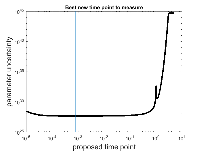
 - Compute the Jacobian matrix at the best estimate
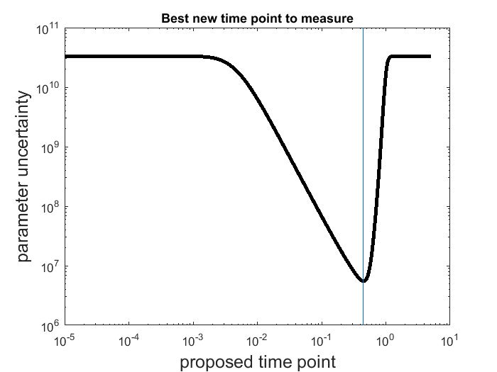
 . Compute the Fisher Information Matrix
  , which is an approximation of the Hessian of the cost function at the current best estimate. Estimate the parameter uncertainty:
 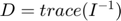 .
. - For each possible new experiment, compute the extended Jacobian, which is the Jacobian in step 2 appended by the partial derivatives of the new data with respect to the parameters. Compute parameter uncertainty based on the extended Jacobians. Suggest the experiment with smallest uncertainty as the next new experiment.
- Carry out the suggested experiment to obtain new data.
- Iterate through steps 1-4 to suggest new experiments until uncertainty cannot be reduced.
In this particular example, let's define the universe of all possible new experiments to be measuring another time point between t=0 and t=5. Since we have already finished step 1 above and obtained an estimate. We will do steps 2-4 here.
% step 2: compute Jacobian for the current experimental design at estimated parameter, and compute uncertainty
J=[];
J(1,:) = (-t_obs(:).*exp(-est_para(1)*t_obs(:)))';
J(2,:) = (-t_obs(:).*exp(-est_para(2)*t_obs(:)))';
uncertainty = sum(1./(svd([J]).^2))  % evalue of J'J is the same as square of singular value of J
uncertainty =

   4.9266e+44
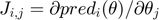
% step 3: for each possible new experiment compute the Jacobian for current+possible experimental design at estimated parameter and compute uncertainty
possible_t = 10.^(-5:(log10(5)+5)/1000:log10(5));
score = zeros(size(possible_t));
for i=1:length(possible_t)
    new_t = unique([t_obs(:);possible_t(i)]);
    new_J = [];
    new_J(1,:) = (-new_t(:).*exp(-est_para(1)*new_t(:)))';
    new_J(2,:) = (-new_t(:).*exp(-est_para(2)*new_t(:)))';
    score(i) = sum(1./(svd([new_J]).^2));
end
[~,ind] = min(score);
t_new = possible_t(ind)
best_new_uncertainty = score(ind)

% visualize the uncertainty across all possible new designs, where we can immediate see a few things that make perfect sense:
%   - early time points are more informative
%   - the flat region after time point t=3 does not decrease uncertainty at all, because t=3 is already too late and too close to 0, any time point after that is unlikely to be useful
%   - the score at time point t=3 is the same as the previous uncertainty, indicating that measuring t=3 again does not help at all
%   - the score at time point t=1 is less than the previous uncertainty (6.1e+44), indicating that measuring t=1 again can help
%   - the score at time point t=1 peaks (bad), showing that measuring the same time point again is less informative than measuring a different time point
close all
loglog(possible_t, score,'k','linewidth',3)
xlabel('proposed time point','Fontsize',15)
ylabel('parameter uncertainty','Fontsize',15)
line(t_new*[1,1], ylim)
title('Best new time point to measure')
t_new =

   8.0067e-04


best_new_uncertainty =

   4.5692e+27
% step 4: now that the best new experiment is selected (t=0.0008), let's actually do it, obtain more data
t_obs = [0.0008;1;3];                           % design of new experiment
true_para = [14;11.5];                          % true parameter
y_obs = toy_system_evaluate(true_para,t_obs);   % obs data if noise free

% back to steps 1 and 2: with new data, we can redo parameter estimation and quantify new uncertainty.
optimization_options = optimoptions(@lsqnonlin,'Algorithm','levenberg-marquardt','MaxFunEvals',1500,'Display','off');
est_para = lsqnonlin(@(x) my_obj_fun(x, y_obs, t_obs), [0;0], [], [], optimization_options); % x is estimated_parameter
est_para
y_pred = toy_system_evaluate(est_para,t_obs);
objective_function_value = sum((y_obs - y_pred).^2)
J=[];
J(1,:) = (-t_obs(:).*exp(-est_para(1)*t_obs(:)))';
J(2,:) = (-t_obs(:).*exp(-est_para(2)*t_obs(:)))';
uncertainty = sum(1./(svd([J]).^2))  % evalue of J'J is the same as square of singular value of J
% Here, after the new time point is added,
%   - the amount of data is increased
%   - the new estimated parameter values are closer to the ground truth
%   - the uncertainty is reduced
est_para =

   13.8543
   11.6454


objective_function_value =

   1.5393e-12


uncertainty =

   3.2973e+10
% Let's do it one more round, and try to ask the experimental design algorith to suggest a fourth time point.
% step 3 again (same code as above): for each possible new experiment compute the Jacobian for current+possible experimental design at estimated parameter and compute uncertainty
possible_t = 10.^(-5:(log10(5)+5)/1000:log10(5));
score = zeros(size(possible_t));
for i=1:length(possible_t)
    new_t = unique([t_obs(:);possible_t(i)]);
    new_J = [];
    new_J(1,:) = (-new_t(:).*exp(-est_para(1)*new_t(:)))';
    new_J(2,:) = (-new_t(:).*exp(-est_para(2)*new_t(:)))';
    score(i) = sum(1./(svd([new_J]).^2));
end
[~,ind] = min(score);
t_new = possible_t(ind)
best_new_uncertainty = score(ind)

% visualize the uncertainty across all possible new designs:
%   - very early time points are no longer very informative, because we already have 0.0008 measured and we know the system starts at x3(t=0)=2
%   - score after t=1 is flat, so now time point between 1 and 3 are not useful any more
%   - the best score occurs at a "gap" time point t=0.46, which is halfway before t=1
close all
loglog(possible_t, score,'k','linewidth',3)
xlabel('proposed time point','Fontsize',15)
ylabel('parameter uncertainty','Fontsize',15)
line(t_new*[1,1], ylim)
title('Best new time point to measure')
t_new =

    0.4471


best_new_uncertainty =

   5.4786e+06
% step 4 again: add the selected fourth time point (t=0.4589),  obtain more data
t_obs = [0.0008;0.4589;1;3];                    % design of new experiment
true_para = [14;11.5];                          % true parameter
y_obs = toy_system_evaluate(true_para,t_obs);   % obs data if noise free

% back to steps 1 and 2: with new data, we can redo parameter estimation and quantify new uncertainty.
optimization_options = optimoptions(@lsqnonlin,'Algorithm','levenberg-marquardt','MaxFunEvals',1500,'Display','off');
est_para = lsqnonlin(@(x) my_obj_fun(x, y_obs, t_obs), [0;0], [], [], optimization_options); % x is estimated_parameter
est_para
y_pred = toy_system_evaluate(est_para,t_obs);
objective_function_value = sum((y_obs - y_pred).^2)
J=[];
J(1,:) = (-t_obs(:).*exp(-est_para(1)*t_obs(:)))';
J(2,:) = (-t_obs(:).*exp(-est_para(2)*t_obs(:)))';
uncertainty = sum(1./(svd([J]).^2))  % evalue of J'J is the same as square of singular value of J
% Here, again, after the new time point is added,
%   - the amount of data is increased
%   - the new estimated parameter values are very close to the ground truth
%   - the uncertainty is further reduced
est_para =

   11.4999
   14.0001


objective_function_value =

   5.1023e-14


uncertainty =

   4.5675e+06
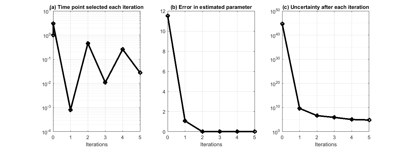
This process can iterate and suggest more data points. We have prepared a separate .m file that encapsulated the above process in a for loop, and asked the algorithm to run 5 iterations. The .m file is available at experiment_design_uncertainty_iterative_process.m. The result is shown in the figure below, where we can see the suggested time points by each iteration, the error in estimated parameters quickly reduce to close to 0, and the reduction of uncertainty along the process.
Experimental design algorithm based on profile likelihood
In this section, we will use the same example to illustrate another experimental design algorithm presented in Steiert B, et al. "Experimental design for parameter estimation of gene regulatory networks", PLoS One. 7(7):e40052, 2012. Steiert et al defined a loglikelihood function for parameter optimization. The likelihood function takes the form of
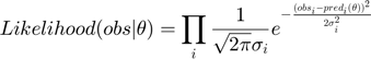
where  represents some form of measurement noise, indicating how much we can trust/use a particular data point. If we are willing to assume that all measurements are equally accurate (
 ), the negative loglikelihood becomes

which is the same as the cost function used in the previous section. The original likelihood function or the negative loglikelihood cost function can be used to define the profile likelihood.
The profile likelihood for each parameter is a function of the parameter, defined by solving many optimization problems. Let's pick parameter as an example. If we fix to be a certain value (e.g. 0.123), we can perform optimization to find the best cost function value and also the estimated values for the other parameters. If we vary the value of across its feasible range and perform the optimization for each possible value of , we will obtain two curves: one is the optimal cost as a scalar function of , and the other is the optimal parameter values as a vector function of . The first of the two curves is the profile likelihood of . The profile likelihood of characterizes what is the best we can do in the optimization problem if is fixed. We can do the same analysis for each parameter, and obtain a collection of  profile likelihoods, where is the number of parameters.
For each profile, for example the likelihood profile of , we can identify the minimal, which indicates the best value to fix , and also define some kind of confidence interval around it. For example a generous definition would be a 90 percentile of the optimized cost function values, which exclude 10 percent of possible values that lead optimized cost function values larger than the threshold. The accepted values and the optimized / estimated values for other parameters form a collection of acceptable parameter setting derived from the likelihood profile of . If we do the same analysis for all likelihood profiles, we will obtain a larger collection of acceptable parameter settings.
These acceptable parameter settings can then be used for experimental design. For one possible experiment, we can use these acceptable parameter settings to simulate the system, and see what is the range of the simulated behavior. If the range is small, all these acceptable parameters lead to similar prediction of the data that will be obtained by the experiment, meaning that this experiment is unlikely to be useful. However, if the range is large, this new experiment will have the ability to differentiate these acceptable parameters, meaning that this experiment is able to further constrain the parameters, and hence informative.
Given this brief introduction of profile likelihood, here is an algorithm procedure for performing experimental design using profile likelihood:
- Compute profile likelihood for each parameter. Basically, pick one parameter and vary its value in the feasible region, and for each value perform optimization to estimate values of other parameters. The optimization objective is a least-squares cost function .
- Define thresholds to obtain the collection of acceptable parameter settings from the profile likelihoods.
- For each possible new experiment, simulate the system using all the acceptable parameter settings, and compute the range of the simulated predictions. Suggest the experiment with largest range as the next new experiment.
- Carry out the suggested experiment to obtain new data.
- Iterate through steps 1-4 to suggest new experiments until some stopping criterion (maybe profile likelihood become very shape, or the range of simulated predictions become very tiny).
Now, let's go through this algorithm using the toy example system here.
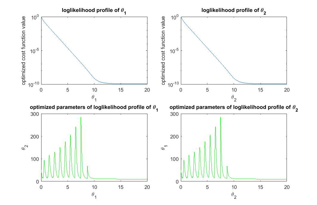
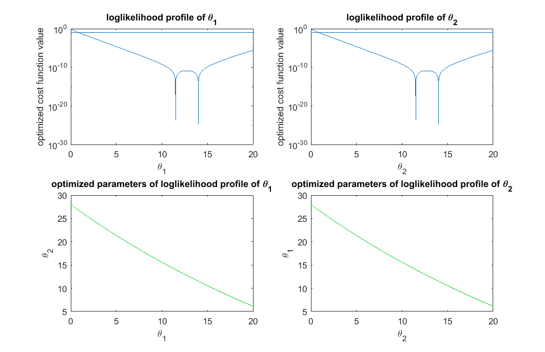
% simulate the initial data, same as before
clear all
t_obs = [1;3];                                  % design of initial experiment
true_para = [14;11.5];                          % true parameter
y_obs = toy_system_evaluate(true_para,t_obs);   % obs data if noise free

% step 1: compute the profile likelihood
theta_range = 0:0.01:20;
likelihood_profile_of_theta_1 = zeros(1,length(theta_range));
est_para_for_profile_of_theta_1 = zeros(2,length(theta_range));
optimization_options = optimoptions(@lsqnonlin,'Algorithm','levenberg-marquardt','MaxFunEvals',1500,'Display','off');
for i=1:length(theta_range)
    theta1 = theta_range(i);
    est_theta2 = lsqnonlin(@(x) my_obj_fun([theta1;x], y_obs, t_obs), [0], [], [], optimization_options); % x is estimated_parameter
    likelihood_profile_of_theta_1(i) = 0.5*sum((y_obs - toy_system_evaluate([theta1;est_theta2],t_obs)).^2);
    est_para_for_profile_of_theta_1(:,i) = [theta1;est_theta2];
end

likelihood_profile_of_theta_2 = zeros(1,length(theta_range));
est_para_for_profile_of_theta_2 = zeros(2,length(theta_range));
optimization_options = optimoptions(@lsqnonlin,'Algorithm','levenberg-marquardt','MaxFunEvals',1500,'Display','off');
for i=1:length(theta_range)
    theta2 = theta_range(i);
    est_theta1 = lsqnonlin(@(x) my_obj_fun([x;theta2], y_obs, t_obs), [0], [], [], optimization_options); % x is estimated_parameter
    likelihood_profile_of_theta_2(i) = 0.5*sum((y_obs - toy_system_evaluate([est_theta1;theta2],t_obs)).^2);
    est_para_for_profile_of_theta_2(:,i) = [est_theta1;theta2];
end

close all
h = figure(1); set(h,'position',[100,100,850,550])
figure(1); subplot(2,2,1); semilogy(theta_range, likelihood_profile_of_theta_1);
xlabel('\theta_1'); ylabel('optimized cost function value'); title('loglikelihood profile of \theta_1')
figure(1); subplot(2,2,2); semilogy(theta_range, likelihood_profile_of_theta_2);
xlabel('\theta_2'); ylabel('optimized cost function value'); title('loglikelihood profile of \theta_2')
figure(1); subplot(2,2,3); plot(est_para_for_profile_of_theta_1(1,:), est_para_for_profile_of_theta_1(2,:),'g-')
xlabel('\theta_1'); ylabel('\theta_2'); title('optimized parameters of loglikelihood profile of \theta_1')
figure(1); subplot(2,2,4); plot(est_para_for_profile_of_theta_2(2,:), est_para_for_profile_of_theta_2(1,:),'g-')
xlabel('\theta_2'); ylabel('\theta_1'); title('optimized parameters of loglikelihood profile of \theta_2')
drawnow
snapnow

% Quick NOTES:
% (1) since the two parameters are symmetric, the profile and optimized
%     parameter values for the two parameters are the same.
% (2) top plot show the likelihood profile. For example, the upper left,
%     when we fix \theta_1 to be a certain value, and optimize the cost
%     function over \theta_2, what is the best cost function for each
%     \theta_1 value.
% (3) bottom plot show the optimized parameter settings. For example, the
%     bottom left, when we fix \theta_1 to be a certain value, and optimize
%     the cost function over \theta_2, what is \theta_2 value that
%     correspond to the best cost function for each \theta_1 value.
% (4) In the upper left plot, the cost function value is large when
%     \theta_1 is small, because when \theta_1 is fixed small, there is no
%     way to tune/optimize \theta_2 to get good cost function value. This
%     also relates to the note (5) below.
% (5) bottom left panel, the strange oscillating pattern is because: when
%     \theta_1 is fixed to be two small, there is no possible \theta_2
%     value that can drive the objective to be small. It is probably
%     numerical issues that generated this strange oscillation pattern.
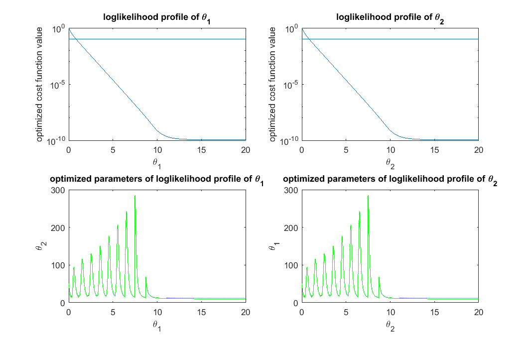
% step 2: define thresholds for acceptable parameters (very generous definition, different from Steiert et al, 2012)
acceptable_est_para = [];
threshold_for_theta_1 = max(exp(-likelihood_profile_of_theta_1))*0.9;
acceptable_indicator_1 = exp(-likelihood_profile_of_theta_1)>=threshold_for_theta_1;
acceptable_est_para = [acceptable_est_para, est_para_for_profile_of_theta_1(:,acceptable_indicator_1)];
threshold_for_theta_2 = max(exp(-likelihood_profile_of_theta_2))*0.9;
acceptable_indicator_2 = exp(-likelihood_profile_of_theta_2)>=threshold_for_theta_2;
acceptable_est_para = [acceptable_est_para, est_para_for_profile_of_theta_2(:,acceptable_indicator_2)];

close all
h = figure(1); set(h,'position',[100,100,850,550])
figure(1); subplot(2,2,1); semilogy(theta_range, likelihood_profile_of_theta_1); line(xlim,[1,1]*(-log(threshold_for_theta_1)))
xlabel('\theta_1'); ylabel('optimized cost function value'); title('loglikelihood profile of \theta_1')
figure(1); subplot(2,2,2); semilogy(theta_range, likelihood_profile_of_theta_2); line(xlim,[1,1]*(-log(threshold_for_theta_2)))
xlabel('\theta_2'); ylabel('optimized cost function value'); title('loglikelihood profile of \theta_2')
figure(1); subplot(2,2,3); plot(est_para_for_profile_of_theta_1(1,:), est_para_for_profile_of_theta_1(2,:),'g-',est_para_for_profile_of_theta_1(1,find(acceptable_indicator_1==1)), est_para_for_profile_of_theta_1(2,find(acceptable_indicator_1==1)),'b.');
xlabel('\theta_1'); ylabel('\theta_2'); title('optimized parameters of loglikelihood profile of \theta_1')
figure(1); subplot(2,2,4); plot(est_para_for_profile_of_theta_2(2,:), est_para_for_profile_of_theta_2(1,:),'g-',est_para_for_profile_of_theta_2(2,acceptable_indicator_2==1), est_para_for_profile_of_theta_2(1,acceptable_indicator_2==1),'b.');
xlabel('\theta_2'); ylabel('\theta_1'); title('optimized parameters of loglikelihood profile of \theta_2')
drawnow
snapnow

% Quick NOTES:
% (1) To define acceptable parameter settings, one needs to decide on an
%     arbitrary threshold. Here, we defined it to be best_likelihood*0.9:
%           max(exp(-likelihood_profile))*0.9;
%     which is fairly generous threshold. One can certainly choose a more
%     strigent threshold, or vary it in the next iteration of the experimental
%     design.
% (2) The horizontal bar in the top plots represent the acceptable
%     threshold of the profile likelihood
% (3) In the bottom plot, the blue dots represent the acceptable parameter
%     settings along the likelihood profile, while the green dots represent
%     parameter settings that are not acceptable according to the
%     threshold.
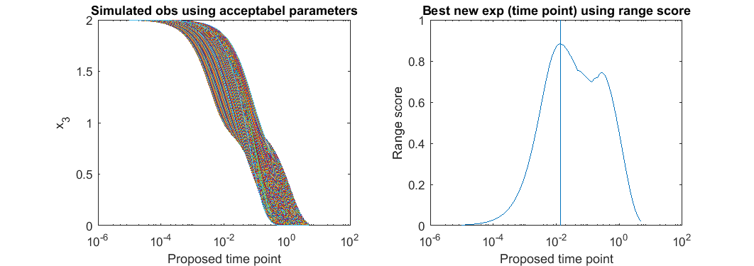
% step 3: For each possible new experiment, simulate the system using all the acceptable parameter settings,
% compute the range of the simulated predictions, and suggest the experiment with largest range.
possible_t = 10.^(-5:(log10(5)+5)/1000:log10(5));
all_simulated_obs=[];
for i=1:size(acceptable_est_para,2)
    simulated_obs = toy_system_evaluate(acceptable_est_para(:,i),possible_t);
    all_simulated_obs = [all_simulated_obs;simulated_obs'];
end
score = max(all_simulated_obs)-min(all_simulated_obs);
[~,ind] = max(score);
t_new = possible_t(ind)

close all
h = figure(1); set(h,'position',[100,100,850,300])
figure(1); subplot(1,2,1); semilogx(possible_t, all_simulated_obs);
xlabel('Proposed time point'); ylabel('x_3'); title('Simulated obs using acceptabel parameters')
figure(1); subplot(1,2,2); semilogx(possible_t, score); line(t_new*[1,1],ylim)
xlabel('Proposed time point'); ylabel('Range score'); title('Best new exp (time point) using range score')
t_new =

    0.0135
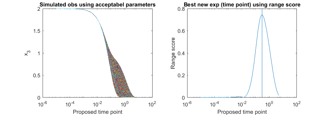
% With this new time point suggested, we can do experimental design all over again and ask for the next time point
t_obs = [0.0128;1;3];                           % design of experiment with 3 time points
true_para = [14;11.5];                          % true parameter
y_obs = toy_system_evaluate(true_para,t_obs);   % obs data if noise free

% step 1: compute the profile likelihood
theta_range = 0:0.01:20;
likelihood_profile_of_theta_1 = zeros(1,length(theta_range));
est_para_for_profile_of_theta_1 = zeros(2,length(theta_range));
optimization_options = optimoptions(@lsqnonlin,'Algorithm','levenberg-marquardt','MaxFunEvals',1500,'Display','off');
for i=1:length(theta_range)
    theta1 = theta_range(i);
    est_theta2 = lsqnonlin(@(x) my_obj_fun([theta1;x], y_obs, t_obs), [0], [], [], optimization_options); % x is estimated_parameter
    likelihood_profile_of_theta_1(i) = 0.5*sum((y_obs - toy_system_evaluate([theta1;est_theta2],t_obs)).^2);
    est_para_for_profile_of_theta_1(:,i) = [theta1;est_theta2];
end

likelihood_profile_of_theta_2 = zeros(1,length(theta_range));
est_para_for_profile_of_theta_2 = zeros(2,length(theta_range));
optimization_options = optimoptions(@lsqnonlin,'Algorithm','levenberg-marquardt','MaxFunEvals',1500,'Display','off');
for i=1:length(theta_range)
    theta2 = theta_range(i);
    est_theta1 = lsqnonlin(@(x) my_obj_fun([x;theta2], y_obs, t_obs), [0], [], [], optimization_options); % x is estimated_parameter
    likelihood_profile_of_theta_2(i) = 0.5*sum((y_obs - toy_system_evaluate([est_theta1;theta2],t_obs)).^2);
    est_para_for_profile_of_theta_2(:,i) = [est_theta1;theta2];
end


% step 2: define thresholds for acceptable parameters (very generous definition, different from Steiert et al, 2012)
acceptable_est_para = [];
threshold_for_theta_1 = max(exp(-likelihood_profile_of_theta_1))*0.9;
acceptable_indicator_1 = exp(-likelihood_profile_of_theta_1)>=threshold_for_theta_1;
acceptable_est_para = [acceptable_est_para, est_para_for_profile_of_theta_1(:,acceptable_indicator_1)];
threshold_for_theta_2 = max(exp(-likelihood_profile_of_theta_2))*0.9;
acceptable_indicator_2 = exp(-likelihood_profile_of_theta_2)>=threshold_for_theta_2;
acceptable_est_para = [acceptable_est_para, est_para_for_profile_of_theta_2(:,acceptable_indicator_2)];

close all
h = figure(1); set(h,'position',[100,100,850,550])
figure(1); subplot(2,2,1); semilogy(theta_range, likelihood_profile_of_theta_1); line(xlim,[1,1]*(-log(threshold_for_theta_1)))
xlabel('\theta_1'); ylabel('optimized cost function value'); title('loglikelihood profile of \theta_1')
figure(1); subplot(2,2,2); semilogy(theta_range, likelihood_profile_of_theta_2); line(xlim,[1,1]*(-log(threshold_for_theta_2)))
xlabel('\theta_2'); ylabel('optimized cost function value'); title('loglikelihood profile of \theta_2')
figure(1); subplot(2,2,3); plot(est_para_for_profile_of_theta_1(1,:), est_para_for_profile_of_theta_1(2,:),'g-',est_para_for_profile_of_theta_1(1,find(acceptable_indicator_1==1)), est_para_for_profile_of_theta_1(2,find(acceptable_indicator_1==1)),'b.');
xlabel('\theta_1'); ylabel('\theta_2'); title('optimized parameters of loglikelihood profile of \theta_1')
figure(1); subplot(2,2,4); plot(est_para_for_profile_of_theta_2(2,:), est_para_for_profile_of_theta_2(1,:),'g-',est_para_for_profile_of_theta_2(2,acceptable_indicator_2==1), est_para_for_profile_of_theta_2(1,acceptable_indicator_2==1),'b.');
xlabel('\theta_2'); ylabel('\theta_1'); title('optimized parameters of loglikelihood profile of \theta_2')
drawnow
snapnow


% step 3: For each possible new experiment, simulate the system using all the acceptable parameter settings,
% compute the range of the simulated predictions, and suggest the experiment with largest range.
possible_t = 10.^(-5:(log10(5)+5)/1000:log10(5));
all_simulated_obs=[];
for i=1:size(acceptable_est_para,2)
    simulated_obs = toy_system_evaluate(acceptable_est_para(:,i),possible_t);
    all_simulated_obs = [all_simulated_obs;simulated_obs'];
end
score = max(all_simulated_obs)-min(all_simulated_obs);
[~,ind] = max(score);
t_new = possible_t(ind)

close all
h = figure(2); set(h,'position',[100,100,850,300])
figure(2); subplot(1,2,1); semilogx(possible_t, all_simulated_obs);
xlabel('Proposed time point'); ylabel('x_3'); title('Simulated obs using acceptabel parameters')
figure(2); subplot(1,2,2); semilogx(possible_t, score); line(t_new*[1,1],ylim)
xlabel('Proposed time point'); ylabel('Range score'); title('Best new exp (time point) using range score')
drawnow
snapnow
t_new =

    0.2899
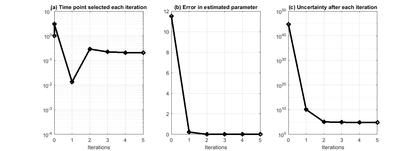
This process can iterate and suggest more data points. We have prepared a separate .m file that encapsulated the above process in a for loop, and asked the algorithm to run 5 iterations. The .m file is available at experiment_design_profile_likelihood_iterative_process.m. The result is shown in the figure below, where we can see the suggested time points by each iteration, the error in estimated parameters quickly reduce to close to 0, same as the experimental design method based on uncertainty reduction. Although profile likelihood does not considered parameter uncertainty, the suggested time points does lead to great reduction of parameter uncertainty along the process.
Geometric interpretation of experimental design
In each experimental design iteration, a new experiment is suggested and performed. More available data means that the dimension of the data space is increased. Since the number of parameter stays the same, the intrinsic dimension of the model manifold does not change. Therefore, increase the data by new experiment will expand the data space by adding new dimensions, and will also deform the manifold into the new dimensions, but will not change the dimension of the manifold.
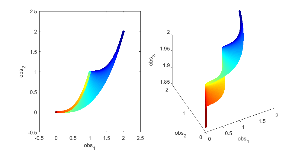
To illustrate this, let's look at a more concrete example using this sum-of-two-exponentials example. With the initial experimental design  , the model manifold is a 2D object (2 parameters) that lives in the 2D data space in the left panel of the figure below. The surface of the model manifold is colored by the sum of the two parameters. The upper right corner (blue) corresponds to both parameters being small. The bottom left corner (red) corresponds to both parameters being large. In the preliminary example, data of the initial experiment sits in the bottom left corner of the manifold. The first iteration of experimental design suggests a third observation x_3(t=0.0007), and the model manifold becomes a 2D object in the 3D data space in the right panel of the figure below, colored in the same way. In the right plot below, if we look at the model manifold in the 3D space from top to down, we will see the exact same figure as the 2D version in the left plot. From the color, we can see that the bottom left corner is expanded and stretched downward (red area becomes larger), while the rest of the model manifold (blue area) is less affected. This is because the new experiment is designed to improve parameter estimation of the data that sits at the bottom left corner. Our conjecture is that the above is true for more complex systems. As the experimental design algorithm iterates, the model manifold is expanded to higher dimension. The manifold region around where the experimental data sits is expanded more than the rest of the manifold.
% Generate many random parameters that will collectively cover the
% parameters space, and hence cover the model manifold
clear all;
K=500000;
para = 10.^(rand(2,K)*6-4);
% define the colors
cmap_tmp = colormap('jet');
color_code_data = sum(log10(para));
prc95 = 3.5;
prc05 = -2.5;
color_code_data = (color_code_data - prc05)/(prc95-prc05);
color_code_data(color_code_data<0.01)=0.01;
color_code_data(color_code_data>0.99)=0.99;
color_code_data = round(color_code_data*100)/100;
node_color = interp1(((1:size(cmap_tmp,1))'-1)/(size(cmap_tmp,1)-1),cmap_tmp,color_code_data);
% plot out the model manifold in the initial 2D data space
close all
h = figure(1); set(h,'position',[100,100,800,400])
t_obs=[1 3]';
y_obs = toy_system_evaluate(para,t_obs);
for i=1:100
    ind = find(round(color_code_data*100)==i);
    if isempty(ind), continue; end
    if i==1, hold off; end
    figure(1); subplot(1,2,1); plot(y_obs(1,ind),y_obs(2,ind),'.','markersize',15,'color',node_color(ind(1),:))
    hold on;
end
% plot out the model manifold in the 3D data space after the first iteration of experimental design
t_obs=[1 3 0.0007]';
y_obs = toy_system_evaluate(para,t_obs);
for i=1:100
    ind = find(round(color_code_data*100)==i);
    if isempty(ind), continue; end
    if i==1, hold off; end
    figure(1); subplot(1,2,2); plot3(y_obs(1,ind),y_obs(2,ind),y_obs(3,ind),'.','markersize',15,'color',node_color(ind(1),:))
    hold on
end
figure(1); subplot(1,2,1); xlabel('obs_1'); ylabel('obs_2'); axis([-0.5,2.5,-0.5,2.5])
figure(1); h = subplot(1,2,2); set(h,'CameraPosition',[ -5,-11, 3]); xlabel('obs_1'); ylabel('obs_2'); zlabel('obs_3')
drawnow
snapnow
Again, as mentioned above, in the right plot, if we look down at the 3D manifold from the top, we should see exactly the same as the left figure. To better appreciate the geometry of the 3D manifold, after running the code above to obtain the figure above, you can use the matlab "Rotate 3D" tool in the figure window to rotate the 3D plot, and get a better understanding of the change in shape. Or alternatively, you can run this .m file on your own computer, experiment_design_change_manifold_shape.m, which generates the following animation that rotates the manifold in 3D data space.
Model reduction problem setup
Model reduction is another strategy to deal with the information gap between a highly complex ODE model in systems biology and a limited amount of experimental data. If we are not able to perform new experiments for some practical reasons (e.g., biological samples are unavailable or experiments are too costly), the data is fixed. In that case, we do not really need a highly complex model to describe the data. We can perform model reduction, and derive reduced models that are able to describe the data with fewer parameters. Furthermore, we can aim for a minimal model that cannot be reduced without losing its ability to fit well to the data, and this minimal model may elucidate the key controlling mechanisms that give rise to the data. The challenge is: there are numerous ways to write down reduced models (e.g., remove or combine parameters or variables). Our model reduction question is: given an ODE model and limited experimental data, how can we systematically derive a sequence of reduced models (each with one fewer degree of freedom), such that the reduced models retain the ability to fit the data? In addition, how can we establish a mathematical justification for the reduced models?
Similar to the experimental design process, the starting point of the model reduction problem is: a mathematical model (description of the systme and description of the experimental data) + the experimentally observed data. Again, the question we want to answer is: given the model and the data, what is the best way to simplify the model. In this setup, the answer to this quesiton is dependent on both the model and the data.
We use the same starting point as the above experimental design examples. Assume the model is as follows, the same equations in the above experimental design examples:
![$$ obs = \left[ \begin{array}{c} x_3(t=1) \\ x_3(t=3) \end{array} \right]$$](publish_model_manifold_eq17726755988142334790.png)
Assume we have performed the experiment and the observed data are and (corresponding to noise-free observation of true underlying parameter ). We would like to perform model reduction based on this starting point.
Different from the matlab examples code in the experimental design section where we took advantage of the analytical solution of this simple toy example to make the code easier, here we use matlab's symbolic capability to provide an implementation that can be easily modified to work with different mathematical models.
Model reduction algorithm based on manifold boundaries
We developed a model reduction algorithm based on manifold boundaries, which we call MBAM, Mark K. Transtrum, Peng Qiu, "Coarse-graining models of emergent behavior by manifold boundaries", Physical Review Letters, 113 (9), 098701, 2014.
The basic idea is to view the experimental data as a point in the data space and identify the nearest manifold boundary. This boundary corresponds to a reduced model with one fewer degree of freedom, and it is able to better fit the data than reduced models corresponding to other boundaries of the manifold.
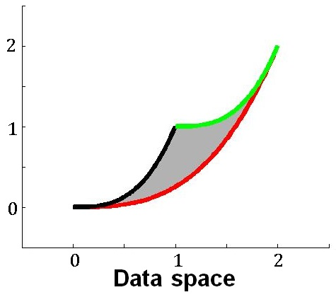
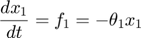
Here is a handwaving illustration of this basic idea. Consider the sum-of-two-exponentials example, the model manifold has three boundaries. (1) If we take to infinity meaning that decays instantaneously, the model reduces to  , and the model manifold becomes a 1D object which is the black boundary indicated in the figure below. (2) If we set to zero meaning x_1 does not decay, the model becomes
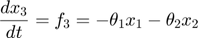
 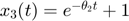 , and its manifold is the green boundary. (3) If the two materials have the same decay rate, the model becomes
 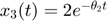 , and its manifold is the red boundary. In this example, manifold boundaries correspond to reduced models that can be derived by physically meaningful limits of the parameters.
The MBAM algorithm is as follows:
- Based on the current model, setup a least-squares cost function for parameter estimation . Perform parameter estimation and obtain the best estimate based on the data.
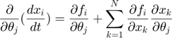
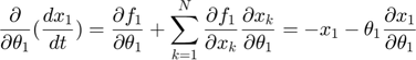
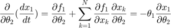
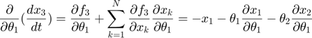
- Identify the manifold boundary nearest to the experimental data by numerical integration of the geodesic equation, which is a set of N nonlinear second order differential equations:
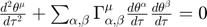 , where
  runs from 1 to N, indexing the parameters.
  is known as the connection coefficient.
 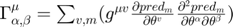 where,
 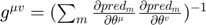 is the
  element of the inverse of the Fisher Information matrix. In the summations,
  run from 1 to the number of parameters N, and
  runs from 1 to the number of experimental observations. If we set
  to be the estimated parameter and set
  to be the eigenvector of the smallest eigenvalue of the Fisher Information matrix (the least sensitive parameter direction), solution to the geodesic equation will be a nonlinear curve in the parameter space which maps to a “straight” line on the manifold, leading to the boundary closest to where the experimental data sits.
 - As the geodesic path approaches a boundary, the Fisher Information matrix becomes singular, and certain parameters approach to limiting values (such as 0, infinity). We evaluate the limits and manually write down the mathematical form of a reduced model.
- With the reduced model, go through steps 1-3 to derive further model reductions, until the reduced model cannot fit the experiment data well.
Since the algorithm uses manifold boundaries to derive reduced models, it requires the model manifold to be bounded, so that boundaries exist. It also requires the model to be differentiable. In systems biology, models are usually constructed with biological assumptions and constraints (such as bounded production, exponential decay, mass conservation, etc.), which make the model manifold bounded. Therefore, MBAM is generally applicable to models in systems biology. The manifold for this toy sum-of-exponentials example is obviously bounded, and hence can be analyzed using MBAM.
The geodesic equation looks complicated. Let's un-complicate it, and spell out the entire set of equations and the numerical solution.
Since the connection coefficient requires the first and second order derivatives of the model predictions (observations) with respece to the parameters, we need a systematic way to compute them. Although we can compute them by finite differences, finite differences can be inaccurate (especially when the geodesic path approaches the manifold boundary). Therefore, we would like to use the sensitivity equations to obtain these derivatives.
In this toy system, the dynamic variables ( ) are functions of time, and their dyanmics (change with respect to time) are governed by the differential equations of the system and their initial conditions. At any time point, we can take the derivative of one dynamic variable with respect to one parameters (e.g.
  ). If we look at this particular derivative at different time point, we will realize that is also a function of time, which we can denote as
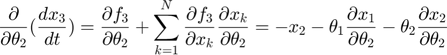
  . In fact, for and other such functions for other variable/parameter combinations, the time dynamics for these functions are also governed by a set of differential equations, which are the sensitivity equations. These sensitivity equations can be derived by taking partial derivatives of both sides of the ODEs with respect to the parameters. For example, if the one ODE is
we can take partial derivative of both sides with respect to one parameter  , and obtain the following equation, where the left hand side is the time derivative of the
  function of time, and itself plus other such
  functions appear on the right hand side.
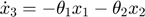
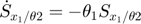
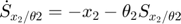
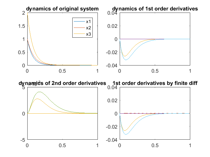
In the toy system, the original model is:

Applying the sensitivity equations to the toy example system, we will have the following:
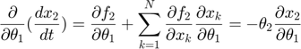
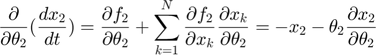
Therefore,the complete set of original + sensitivity equations are:


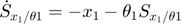


To be able to numerically solve this newer extended set of ODEs, we will also need initial conditions. The initial conditions of  varlables are given in the original model. The initial conditions of
  variables can be obtained by taking the derivatives of the initial conditions of with respect to the parameters. The initial conditions of are all trivially 0 in this example. However, in cases where some the initial conditions of the origial system contains parameters or are themselves parameters, the initial conditions of will not be 0. Initial conditions of this extended set of ODEs are:


This can be further extended to obtain the ODEs that govern the time dynamics of second order derivatives of the dynamic variables with respect to the parameters.
The sensitivity equations can be computed in matlab using its symbolic capability. In the Necesary Function section on this page, we provide a function that computes/generates the sensitivity equations without the need for any hand calculation. Below shows one example of how to use it.
% define name/symbol of the variables
x = [sym('x1'); ...
     sym('x2');...
     sym('x3');...
     ];

% define name/symbol of parameters
theta = [sym('theta1'); ...
         sym('theta2');...
        ];

% define the right-hand-side of the ODE equations
dx = [-theta(1) * x(1); ...
      -theta(2) * x(2); ...
      -theta(1) * x(1) - theta(2) * x(2); ...
      ];

% define initial conditions of x
x0     = [sym('1');...
          sym('1');...
          sym('2');...
         ];

% dimension of the problem
M=length(x);        % number of dynamic variables
N=length(theta);    % number of parameters

% define observation configuration. Each row is one observation.
% First column indicates which variable observed.
% Second column is time point.
obs_config = [3, 1; ...
              3, 3; ...
             ];   %In this eg, we observe x3 at time points 1,3


% construct an geodesic object of the ODEgeodesics class
obj = ODEgeodesics(x, dx, x0, theta, obs_config);


% compare the following three to the original system model:
disp('system dynamic variables:')
disp(obj.x)
disp('ODE right hand side:')
disp(obj.dx)
disp('initial conditions:')
disp(obj.x0)


% compute 1st order sensitivity, needed for integrating geodesics
obj = obj.compute_1st_order_sensitivity_equations;


% compare the following three to the sensitity equations above:
disp('variables for the 1st order derivatives:')
disp(obj.S)
disp('1st order sensitivity equation ODE right hand side:')
disp(obj.dS)
disp('1st order sensitivity initial conditions:')
disp(obj.S0)

% compute 2nd order sensitivity
obj = obj.compute_2nd_order_sensitivity_equations;              % only needed if we set obj.accerlation_compute_opt = '2nd_order_sensitivity_for_Gamma';

% the 2nd order sensitivity equations are more extensive. you can view them using the following 6 lines that are commented out
% disp('variables for the 2nd order derivatives:')
% disp(obj.SS)
% disp('2nd order sensitivity equation ODE right hand side:')
% disp(obj.dSS)
% disp('2nd order sensitivity initial conditions:')
% disp(obj.SS0)
system dynamic variables:
 x1
 x2
 x3

ODE right hand side:
              -theta1*x1
              -theta2*x2
 - theta1*x1 - theta2*x2

initial conditions:
 1
 1
 2

variables for the 1st order derivatives:
[ dx1_dtheta1, dx1_dtheta2]
[ dx2_dtheta1, dx2_dtheta2]
[ dx3_dtheta1, dx3_dtheta2]

1st order sensitivity equation ODE right hand side:
[                      - x1 - dx1_dtheta1*theta1,                            -dx1_dtheta2*theta1]
[                            -dx2_dtheta1*theta2,                      - x2 - dx2_dtheta2*theta2]
[ - x1 - dx1_dtheta1*theta1 - dx2_dtheta1*theta2, - x2 - dx1_dtheta2*theta1 - dx2_dtheta2*theta2]

1st order sensitivity initial conditions:
[ 0, 0]
[ 0, 0]
[ 0, 0]
So far, everything above is symbolic. Now, let's use these symbolic ODEs to get some real numbers.
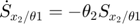
% simulate the model with the above parameters
para = [14, 11.5]';
time_points_to_plot = [0:0.01:4];
[t,y] = ode45(@(t,x_values)obj.ODE_rhs(t,x_values,para),[time_points_to_plot],obj.ODE_init(para));  % numerically integrate, evaluate at the observed time points. Important to add 0 as the first time point, because ODE45 views the first time point as the time of the initial condition
% simulate the model with slightly changed parameters
para1 = para; para1(1) = para1(1)+0.001;
para2 = para; para2(2) = para1(2)+0.001;
[t,y1] = ode45(@(t,x_values)obj.ODE_rhs(t,x_values,para1),[time_points_to_plot],obj.ODE_init(para1));
[t,y2] = ode45(@(t,x_values)obj.ODE_rhs(t,x_values,para2),[time_points_to_plot],obj.ODE_init(para2));
% simulate the model and 1st and 2nd order sensitivity equations
[t,y_1st_2nd] = ode45(@(t,x_values)obj.ODE_2nd_order_sensitivity_rhs(t,x_values,para),[time_points_to_plot],obj.ODE_2nd_order_sensitivity_init(para));  % numerically integrate, evaluate at the observed time points. Important to add 0 as the first time point, because ODE45 views the first time point as the time of the initial condition

% plot the simulation results
close all
figure(1)
subplot(2,2,1); plot(t,y(:,1:3)); legend({'x1','x2','x3'});xlim([0,1]); title('dynamics of original system');
subplot(2,2,2); plot(t,y_1st_2nd(:,4:9)); xlim([0,1]); ylim([-0.04,0.04]); title('dynamics of 1st order derivatives');
subplot(2,2,3); plot(t,y_1st_2nd(:,10:end)); xlim([0,1]); ylim([-0.005,0.005]); title('dynamics of 2nd order derivatives');
subplot(2,2,4); plot(t,[y1(:,1:3)-y(:,1:3), y2(:,1:3)-y(:,1:3)]/0.001); xlim([0,1]); ylim([-0.04,0.04]); title('1st order derivatives by finite diff');
drawnow
snapnow
In the figure above, the upper-left shows the dynamics of 3 system variables. The upper-right shows the dynamics of the first order derivatives computed by sensitivity equations, which are atually 6 curves:  and
and  are identical,
  and
and  are identical,
  and
and  are constant 0. The bottom-right are also the first order derivatives, but computed by finite difference, which agrees well with the upper-right. The bottom-left are the second order derivatives computed by sensitivity equations, which are a total of 3*3*2 = 12 curves: many are constant 0, 2 show identical dynamics, 2 show another identical dynamics.
With such a sensitivity equation implementation, we are able to conveniently evaluate the first and second order derivatives of the variables with respect to the parameters at any time point we want, just by numerically solving a (potentially very large) set of ODEs. These derivatives are needed to construct and integrate the geodesic equations.
Since the geodesic equation involve second order time derivatives, we need to turn it into a first order system, before we can use regular matlab ODE solvers to solve the geodesic equation. The second order form is:
Turning the geodesic equations into first order form, we will obtain the following set of equations:
Denote  as
as  , the equations look cleaner, and become the following, where each "[...]" represents one variable in the first order system version of the geodesic equations.
![$$ \dot{[\theta^\mu]} = [d\theta^\mu], \mu = 1,2,...,N$$](publish_model_manifold_eq05834817173734297960.png)
![$$ \dot{[d\theta^\mu]} = - \sum_{\alpha,\beta} \Gamma_{\alpha,\beta}^\mu [d\theta^\alpha] [d\theta^\beta], \mu = 1,2,...,N$$](publish_model_manifold_eq17430246603145312213.png)
In this toy system, the process of solving geodesic path is not very easy, because we do not have the analytical form of the connection coefficient as a function of the parameters  , and can only numerically compute the connection coefficient. Therefore, the process is basically the following: first specify the starting parameter value and an initial velocity (initial conditions of
  and
and  ), compute the connection coefficient at the initial condition of
  , inch forward both and using Euler formula, recompute the connection coefficient at the new , inch foward again, keep repeating this process to obtain the geodesic path in the parameter space. We have implemented this in the ODEgeodesics class. Below is an example.
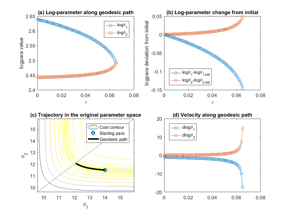
% although MBAM usually start from data and estimate the parameters, in
% this example, let's assume the estimation is perfect, and start with the
% true underlying parameter value

obj = ODEgeodesics(x, dx, x0, theta, obs_config);                       % construct the object
obj.para = [14, 11.5]';                                                 % set initial parameter value
obj = obj.compute_1st_order_sensitivity_equations;                      % compute 1st order sensitivity, needed for integrating geodesics
obj = obj.compute_2nd_order_sensitivity_equations;                      % only needed if we set obj.accerlation_compute_opt = '2nd_order_sensitivity_for_Gamma';
obj.integrate_method_opt = 'Euler';                                     % 'Euler' or 'ODE_solver'(preferred)
obj.accerlation_compute_opt = '2nd_order_sensitivity_for_Gamma';        % '2nd_order_finite_difference' or '2nd_order_sensitivity_for_Gamma'(preferred)
obj.smallest_singular_threshold = 1e-20;                                % need some tuning for different models
obj.check_flipping_acceleration = 1;                                    % useful to guard against overshoot near symmetries
obj.display_integration_process = 0;
[geodesic_path, tau] = obj.numerical_integrate_for_geodesic_path;       % integrate the geodesic path


close all
figure(1)
subplot(2,2,1); plot(tau,geodesic_path(:,1:2),'o-'); legend({'\theta_1','\theta_2'}); xlabel('\tau'); ylabel('para value')
subplot(2,2,2); plot(tau,geodesic_path(:,1:2) - geodesic_path(1,1:2), 'o-'); legend({'\theta_1-\theta_{1,init}','\theta_2-\theta_{2,init}'}, 'location', 'southwest'); xlabel('\tau'); ylabel('para change from initial');
subplot(2,2,3); hold off; sum_exp_parameter_landscape(geodesic_path(1,1:2)',obs_config, geodesic_path(:,1:2)')
 hold on; plot(geodesic_path(1,1),geodesic_path(1,2),'o',geodesic_path(:,1),geodesic_path(:,2),'-k','linewidth',3); line([0,20],[0,20])
 axis_min = min(min(geodesic_path(:,1:2)-max(max(abs(geodesic_path(1,1:2)-geodesic_path(:,1:2))))));
 axis_max = max(max(geodesic_path(:,1:2)+max(max(abs(geodesic_path(1,1:2)-geodesic_path(:,1:2))))));
 axis([axis_min axis_max axis_min axis_max])
 xlabel('\theta_1'); ylabel('\theta_2')
subplot(2,2,4); hold off; plot(tau,geodesic_path(:,3:4),'o-'); title('velocity of para'); legend({'d\theta_1','d\theta_2'}, 'location', 'northwest');ylim([-100,100])
may need to stop, acceleration direction flip
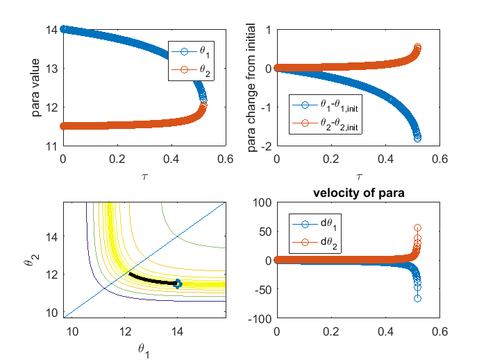
In the example above, we start with initial parameter ![$\theta^\mu = [14, 11.5]'$](publish_model_manifold_eq01138271686427602283.png) . The initial velocity for is the least sensitive parameter direction with respect to the cost function. The initial velocity can be defined by the following procedure: compute the Jacobian matrix
. The initial velocity for is the least sensitive parameter direction with respect to the cost function. The initial velocity can be defined by the following procedure: compute the Jacobian matrix  at the initial parameter setting, compute the fisher information matrix
  , find its eigenvalue and eigenvectors, and the eigenvector corresponding to the smallest eigenvalue is the initial velocity direction. Equivalently, the initial velocity can be defined by the right singular vector of that corresponds to 's smallest singular value. The eigenvector (or the singular vector) is not the initial velocity yet, there is still ambiguity about the direction, because the opposite direction of an eigenvector is also an eigenvector corresponding to the same eigenvalue. Same arguement applies to the singular vector. To determine the direction, we compute the right hand side of the
 ![$\dot{[d\theta^\mu]}$](publish_model_manifold_eq03808218013080316826.png) equation above, which defines the accelerlation. If the inner product of the eigenvector and the acceleration is positive, we define the initial velocity to be the eigenvector. If the inner product is negative, we define the initial velocity to be the negative of the eigenvector. In this case, the initial velocity is [-0.997, 0.081]. The upper left plot shows the trajectory obtained by integrating the geodesic equation, the parameter values as a function of
equation above, which defines the accelerlation. If the inner product of the eigenvector and the acceleration is positive, we define the initial velocity to be the eigenvector. If the inner product is negative, we define the initial velocity to be the negative of the eigenvector. In this case, the initial velocity is [-0.997, 0.081]. The upper left plot shows the trajectory obtained by integrating the geodesic equation, the parameter values as a function of  which parameterizes the geodesic path, where we can see that the two parameters gradually approach each other and become almost the same. In the bottom left plot, we show the geodesic path in the parameter space, overlaid with the cost surface. We can see that the geodesic path started from the initial parameter we specified, and move along the canyon of the cost surface until some limit is achieved. In this case, the limit involves two parameters, which is indicated in the bottom right plot, where the acceleration of two parameters grow very large. Looking at the upper left plot, we can see that the two parameters converge to the same value, which correspond to a symmetry of the model. Therefore, in this particular example, the geodesic path, starting from the initial parameter, following the canyon of the cost surface along the accelerating direction, leads to a limit where the two parameters are the same, which corresponds to one boundary of the model manifold and suggests that an appropriate reduced model should be .
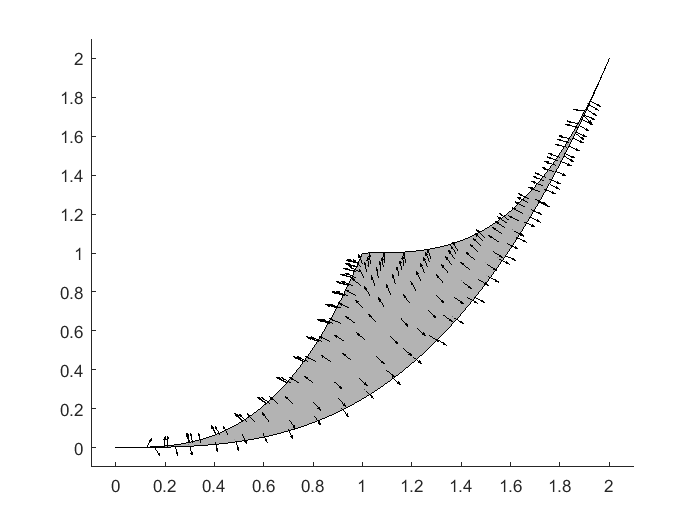
After seeing one geodesic path in the parameter space, the natural next question is how about its corresponding image in the data space on the model manifold? How does the geodesic path look like if we start from other starting points? In below, we provide an example using our code to generate a vector/direction field, displaying the direction of the geodesic paths on the model manifold. From this vector field, it is easy to imagine the trajectory of the geodesic paths on this particular example of model manifold.
close all
figure(2); hold off
theta_tmp=20:-0.01:0;
y1_tmp = [exp(-theta_tmp*1), 1+exp(-theta_tmp*1), fliplr(2*exp(-theta_tmp*1))];
y2_tmp = [exp(-theta_tmp*3), 1+exp(-theta_tmp*3), fliplr(2*exp(-theta_tmp*3))];
patch(y1_tmp,y2_tmp,[0.7,0.7,0.7])
axis([-0.1 2.1 -0.1 2.1])

logtheta1_grid = -4:0.3:2;
logtheta2_grid = -4:0.3:2;
theta1_grid = exp(logtheta1_grid);
theta2_grid = exp(logtheta2_grid);
tmp1 = repmat(theta1_grid(:)',length(theta2_grid),1); tmp1 = tmp1(:);
tmp2 = repmat(theta2_grid(:), 1,length(theta1_grid)); tmp2 = tmp2(:);
warning off;
for i=1:length(tmp1)
    para = [tmp1(i), tmp2(i)]';
    [para_direction, para_acceleration, singular_values] = compute_initial_velocity(obj, para);
    if min(singular_values)<1e-3
        continue;
    end
    y_obs = toy_system_evaluate(para,obs_config(:,2));
    y_new = toy_system_evaluate(para + para_direction*0.01,obs_config(:,2));
    y_direction = (y_new-y_obs)/norm(y_new-y_obs)/20;
    hold on
    plot(y_obs(1),y_obs(2),'k.')
    quiver(y_obs(1),y_obs(2),y_direction(1),y_direction(2),'-k','MaxHeadSize',50, 'AutoScale','off')
end

In this particular example, the parameters are supposed to be non-negative. In systems biology, the construction of many models require parameters to be non-negative. In our example So far, we have not yet considered the non-negative constraint. However, when the geodesic path leads to a boundary corresponding to parameters approaching to 0, the numerical integration process may take the geodesic path out of the feasible parameter region. For non-negative constraints on parameters, one neat trick is to modify the model and work with log-parameters, where we do not have any constraints on the log-parameters and the exponentiation automatically takes care the non-negative constraint.
Below, we show the same example above working with log-parameters.
clear all

% define name/symbol of the variables
x = [sym('x1'); ...
     sym('x2');...
     sym('x3');...
     ];

% define name/symbol of parameters
theta = [sym('logtheta1'); ...
         sym('logtheta2');...
        ];

% define the right-hand-side of the ODE equations
dx = [-exp(theta(1)) * x(1); ...
      -exp(theta(2)) * x(2); ...
      -exp(theta(1)) * x(1) - exp(theta(2)) * x(2); ...
      ];

% define initial conditions of x
x0     = [sym('1');...
          sym('1');...
          sym('2');...
         ];

% dimension of the problem
M=length(x);        % number of dynamic variables
N=length(theta);    % number of parameters

% define observation configuration. Each row is one observation.
% First column indicates which variable observed.
% Second column is time point.
obs_config = [3, 1; ...
              3, 3; ...
             ];   %In this eg, we observe x3 at time points 1,3


% integrate and solve one geodesic path
obj = ODEgeodesics(x, dx, x0, theta, obs_config);                       % construct the object
obj.para = [log(14), log(11.5)]';                                       % set initial parameter value, in log space now
obj = obj.compute_1st_order_sensitivity_equations;                      % compute 1st order sensitivity, needed for integrating geodesics
obj = obj.compute_2nd_order_sensitivity_equations;                      % only needed if we set obj.accerlation_compute_opt = '2nd_order_sensitivity_for_Gamma';
obj.integrate_method_opt = 'Euler';                                     % 'Euler' or 'ODE_solver'(preferred)
obj.accerlation_compute_opt = '2nd_order_sensitivity_for_Gamma';        % '2nd_order_finite_difference' or '2nd_order_sensitivity_for_Gamma'(preferred)
obj.smallest_singular_threshold = 1e-20;                                % need some tuning for different models
obj.check_flipping_acceleration = 1;                                    % useful to guard against overshoot near symmetries
obj.display_integration_process = 0;
[geodesic_path, tau] = obj.numerical_integrate_for_geodesic_path;       % integrate the geodesic path

close all
h = figure(1);  set(h, 'position', [100 100 800 600])
subplot(2,2,1); plot(tau,geodesic_path(:,1:2),'o-'); legend({'log\theta_1','log\theta_2'}); xlabel('\tau'); ylabel('logpara value'); title('(a) Log-parameter along geodesic path')
subplot(2,2,2); plot(tau,geodesic_path(:,1:2) - geodesic_path(1,1:2), 'o-'); legend({'log\theta_1-log\theta_{1,init}','log\theta_2-log\theta_{2,init}'}, 'location', 'southwest'); xlabel('\tau'); ylabel('logpara deviation from initial'); title('(b) Log-parameter change from initial')
subplot(2,2,3); hold off; sum_exp_parameter_landscape(exp(geodesic_path(1,1:2)'),obs_config, exp(geodesic_path(:,1:2))')
 hold on; plot(exp(geodesic_path(1,1)),exp(geodesic_path(1,2)),'o',exp(geodesic_path(:,1)),exp(geodesic_path(:,2)),'-k','linewidth',3); line([0,20],[0,20])
 axis_min = min(min(exp(geodesic_path(:,1:2))-max(max(abs(exp(geodesic_path(1,1:2))-exp(geodesic_path(:,1:2)))))));
 axis_max = max(max(exp(geodesic_path(:,1:2))+max(max(abs(exp(geodesic_path(1,1:2))-exp(geodesic_path(:,1:2)))))));
 axis([axis_min axis_max axis_min axis_max])
 xlabel('\theta_1'); ylabel('\theta_2')
 title('(c) Trajectory in the original parameter space')
 legend({'Cost contour','Starting para','Geodesic path'})
subplot(2,2,4); hold off; plot(tau,geodesic_path(:,3:4),'o-');  legend({'dlog\theta_1','dlog\theta_2'}, 'location', 'northwest'); title('(d) Velocity along geodesic path');
drawnow
snapnow

% show vector/directin field on manifold
close all
figure(2);
theta_tmp=20:-0.01:0;
y1_tmp = [exp(-theta_tmp*1), 1+exp(-theta_tmp*1), fliplr(2*exp(-theta_tmp*1))];
y2_tmp = [exp(-theta_tmp*3), 1+exp(-theta_tmp*3), fliplr(2*exp(-theta_tmp*3))];
patch(y1_tmp,y2_tmp,[0.7,0.7,0.7])
axis([-0.1 2.1 -0.1 2.1])

logtheta1_grid = -4:0.3:2;
logtheta2_grid = -4:0.3:2;
tmp1 = repmat(logtheta1_grid(:)',length(logtheta2_grid),1); tmp1 = tmp1(:);
tmp2 = repmat(logtheta2_grid(:), 1,length(logtheta1_grid)); tmp2 = tmp2(:);
warning off;
for i=1:length(tmp1)
    logpara = [tmp1(i), tmp2(i)]';
    [logpara_direction, logpara_acceleration, singular_values] = compute_initial_velocity(obj, logpara);
    if min(singular_values)<1e-3
        continue;
    end
    y_obs = toy_system_evaluate(exp(logpara),obs_config(:,2));
    y_new = toy_system_evaluate(exp(logpara + logpara_direction*0.01),obs_config(:,2));
    y_direction = (y_new-y_obs)/norm(y_new-y_obs)/20;
    hold on
    plot(y_obs(1),y_obs(2),'k.')
    quiver(y_obs(1),y_obs(2),y_direction(1),y_direction(2),'-k','MaxHeadSize',50, 'AutoScale','off')
end
may need to stop, acceleration direction flip
Comparing the trajectory obtained by working with the origianl parameters and the results from working with log-parameters, we can see that the geodesic path in the parameter space look almost the same, following the canyon of cost surface and graduate approach to the same limit of two parameters being the same.
Comparing the two vector/direction fields on the manifold, we can see that the result look different. This is because the log opertation induces a nonlinear deformation in the parameter space (metric space) that parameterizes the model manifold, which changes the notion of distances. Looking at the two vector fields, it seems that the result from log-parameter space is better, because (1) the notion of distance and closest boundary agrees more with our intuition, (2) there is no need to worry about the non-negative constraints on the parameters. In fact, we would like to argue that the original parameter space is badly distorted because it is much easier to get to the limit of 0 and the limit of infinite is very far away. The log operation removes / compensates the distortion, making it equally easy/difficult to get to the two limits.
Overall, when facing one-side constraints such as the non-negative constraint here, we would always recommend working with log-paramteers in our geodesic path manifold boundary analysis.
After the first iteration of MBAM, the model reduces to 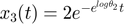 with only one parameter. If we perform a second iteration of MBAM with for example the initial log-parameter
  , the initial velocity is
  , and the geodesic path leads to the limit of
  . Evaluating this limit further reduces the model to a constant of
  , which corresponds to the bottom-left corner of the original model manifold.
Model reduction algorithm based on profile likelihood
The profile likehihood apporach for experimental design can also be applied for model reduction, as discussed in the following paper: Tim Maiwald, et al, "Driving the Model to Its Limit: Profile Likelihood Based Model Reduction", PLoS ONE, 11(9):e0162366, 2016. This idea is actually closely related to our method using manifold boundaries, but there are also some noted differences. We will use the toy exmaple here to discuss the profile likelihood method for model reduction.
As mentioned above in the experimental design sections, the profile likelihood for each parameter is a function of the parameter, defined by solving many optimization optimization problem. Take parameter as an example. We can vary the value of , and for each value, optimize the cost function to obtain estimate of the other parameter. This process will produce two functions: (1) the optimal cost as a scalar function of , and (2) the optimal parameter values as a vector function of . The first of the two functions is the profile likelihood of . We can do the same analysis for each parameter, and obtain a collection of profile likelihoods, where is the number of parameters.
Same as before, for each profile, we can identify the minimal which indicates the best value to fix the parameter, and also define some kind of threshold for acceptable range of this parameter. For example a generous definition would be a 90 percentle of the optimized cost function values, same as before.
Looking at the shape of each profile, we can see when the parameter values achieve its limit (e.g. 0 or inf) on either end of the profile, does the profile go above the threshold. If both side go above, the parameter is considered as identifiable and cannot be removed. If both sides stay below, the parameter is totally unidentifiable, and can be fixed to an arbitrary value. If only one side stay below, that side correspond to a parameter limit that can be used to simplify the model.
Here is a simplified procedure for model reduction using the profile likelihood:
- Compute profile likelihood for each parameter. Pick one parameter and vary its value in the feasible region, and for each value perform optimization to estimate values of other parameters. The optimization objective is a least-squares cost function .
- Define thresholds for acceptable likelihoods.
- Examine the shapes of the profiles with respect to the threshold and decide on the limits to simplify the model. If both ends of a profile exceed the threshold, the corresponding parameter is considered to be identifiable and thus cannot be reduced. If neither ends of a profile exceed the threshold, the corresponding parameter is unidentifiable and can be fixed to an arbitrary value. If one end exceeds the threshold and the other stays below it, the corresponding parameter can be taken to the limit associated to the end that stays below the threshold.
Now, let's go through this algorithm using the toy example system here. The code is essentially the same as before.
% simulate the initial data, same as before
clear all
t_obs = [1;3];                                  % design of initial experiment
true_para = [14;11.5];                          % true parameter
y_obs = toy_system_evaluate(true_para,t_obs);   % obs data if noise free

% step 1: compute the profile likelihood
theta_range = 0:0.01:20;
likelihood_profile_of_theta_1 = zeros(1,length(theta_range));
est_para_for_profile_of_theta_1 = zeros(2,length(theta_range));
optimization_options = optimoptions(@lsqnonlin,'Algorithm','levenberg-marquardt','MaxFunEvals',1500,'Display','off');
for i=1:length(theta_range)
    theta1 = theta_range(i);
    est_theta2 = lsqnonlin(@(x) my_obj_fun([theta1;x], y_obs, t_obs), [0], [], [], optimization_options); % x is estimated_parameter
    likelihood_profile_of_theta_1(i) = 0.5*sum((y_obs - toy_system_evaluate([theta1;est_theta2],t_obs)).^2);
    est_para_for_profile_of_theta_1(:,i) = [theta1;est_theta2];
end

likelihood_profile_of_theta_2 = zeros(1,length(theta_range));
est_para_for_profile_of_theta_2 = zeros(2,length(theta_range));
optimization_options = optimoptions(@lsqnonlin,'Algorithm','levenberg-marquardt','MaxFunEvals',1500,'Display','off');
for i=1:length(theta_range)
    theta2 = theta_range(i);
    est_theta1 = lsqnonlin(@(x) my_obj_fun([x;theta2], y_obs, t_obs), [0], [], [], optimization_options); % x is estimated_parameter
    likelihood_profile_of_theta_2(i) = 0.5*sum((y_obs - toy_system_evaluate([est_theta1;theta2],t_obs)).^2);
    est_para_for_profile_of_theta_2(:,i) = [est_theta1;theta2];
end


% step 2: define thresholds for acceptable parameters (very generous definition, different from Steiert et al, 2012)
threshold_for_theta_1 = max(exp(-likelihood_profile_of_theta_1))*0.9;
threshold_for_theta_2 = max(exp(-likelihood_profile_of_theta_2))*0.9;
close all
h = figure(1); set(h,'position',[100,100,850,350])
figure(1); subplot(1,2,1); semilogy(theta_range, likelihood_profile_of_theta_1); line(xlim,[1,1]*(-log(threshold_for_theta_1)))
xlabel('\theta_1'); ylabel('optimized cost function value'); title('loglikelihood profile of \theta_1')
figure(1); subplot(1,2,2); semilogy(theta_range, likelihood_profile_of_theta_2); line(xlim,[1,1]*(-log(threshold_for_theta_2)))
xlabel('\theta_2'); ylabel('optimized cost function value'); title('loglikelihood profile of \theta_2')
drawnow
snapnow


% step 3: Look at the profiles, and conclude that both parameters can be taken to the limit of Inf
% see discussion right after the figure below.
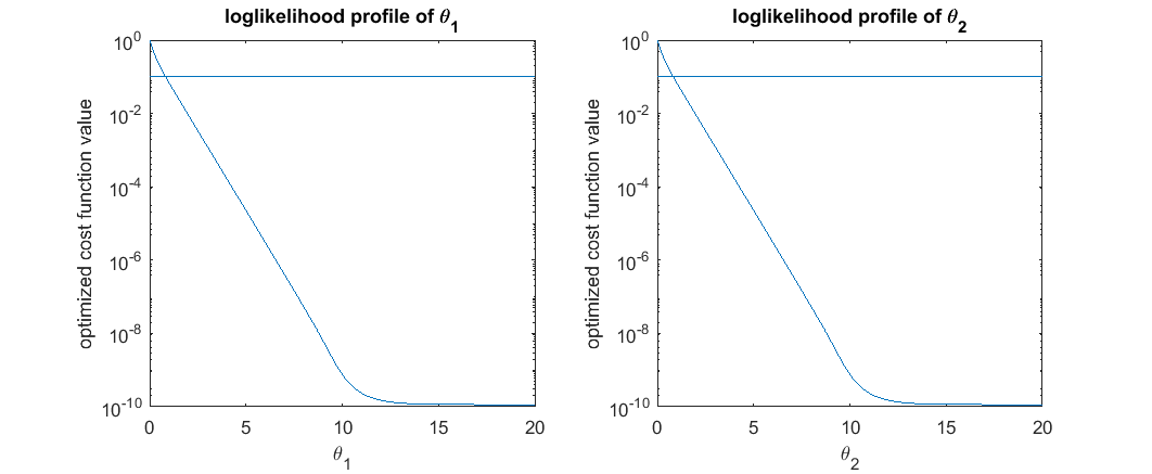
The limits suggested by profile likelihood here are quite good suggestions for model reduction in this example. The reduced model is basically  , which is a constant model without any parameters. This is a quite reasonoable reduced model for the toy example. Because the observed data here are
  and
and  , both very close to 0, the constant reduce model is still able to fit to the data quite well.
Remarks on the two model reduction algorithms
As shown in this example, both manifold boundary and profile likelihood methods perform model reduction by generating parameter trajectories that follow canyons in the cost surface, and both algorithms generate reasonable reduced models.
One key difference between the two algorithms is the computational complexity. The manifold boundary methods involves computation of the connection coefficient along the geodesic path, which requires calculation or approximation of the first- and second-order derivatives of the model predictions with respect to the parameters. This means MBAM requires evaluation of the model and its sensitivities many times along the geodesic path. On the other hand, the profile likelihood is a lot more computationally expensive. Computing the profile likelihood requires performing optimization of the cost function many times, with one parameter fixed at various values to obtain one profile. Each run of optimization involves evaluating the model many times, and can also involve first-order derivatives depending on the optimization algorithm. Therefore, MBAM is more computationally efficient compared to profile likelihood.
Another key difference between the two algorithms is whether parameter combinations are considered. The profile likelihood can identify limits that involve taking individual parameters to their limits ( or
or  ), and can also identify parameter combinations that goes to infinity together. However, profile likelihood is not able to identify limits related to symmetry in the system, for example the limit of
  in the sum-of-two-exponentials example here. This kind of symmetry is actually quite common in systems biology and also in other engineering practices. For example, nearly all machine learning models in regression analysis and neural networks have lots of internal symmetries.
A slightly larger example for model reduction
The sum-of-two-exponential model is a very simple example for model reduction, with only two parameters. In the following link, we provide a slightly more complex example to better illustrate the model reduction algorithm, publish_MBAM_example.html.
Necessary functions
To run the script on this page. You will need to download each function below and save in separate .m files. In below, we also include the code of these functions on this webpage.
--------------------------------------------------------------------------------------------------------------------------------------------------------------------------------------------------------------------------------------------------------------------------------------------------------------------------------------------------------------------------------------------------------------------------------------------------------------------------------------------------------------------------------
% Simulate/evaluate the system using its analytical solution. Typically, this is done by simulating the ODE using solvers such as ode15s, ode45, etc. Because this system is simple enough to allow an analytical solution, the simulation/evaluation is easy.
function obs = toy_system_evaluate(para,t)

    if length(para)==2
        para = para(:);
    end

    N = size(para,2);

    for i=1:N
        theta1 = para(1,i);
        theta2 = para(2,i);
        for j=1:length(t)
            obs(j,i) = exp(-theta1*t(j)) + exp(-theta2*t(j));
        end
    end

end
--------------------------------------------------------------------------------------------------------------------------------------------------------------------------------------------------------------------------------------------------------------------------------------------------------------------------------------------------------------------------------------------------------------------------------------------------------------------------------------------------------------------------------
% Given a set of grid points that form a patch in 2D (boundary and interior), how to find boundarie points with the correct ordering so that the patch function can be used to draw this region.
function outer_points = get_outer_points(grid_position, indicators, delta_x, delta_y)

    patch_squareform = reshape(indicators,sqrt(length(indicators)), sqrt(length(indicators)));
    contour_squareform = zeros(size(patch_squareform));

    for i=1:size(patch_squareform,1)
        ind_tmp = (patch_squareform(i,:)~=[-1,patch_squareform(i,1:end-1)] | patch_squareform(i,:)~=[patch_squareform(i,2:end),-1]) & patch_squareform(i,:)==1;
        contour_squareform(i,ind_tmp)=1;
    end
    for j=1:size(patch_squareform,2)
        ind_tmp = (patch_squareform(:,j)~=[-1;patch_squareform(1:end-1,j)] | patch_squareform(:,j)~=[patch_squareform(2:end,j);-1]) & patch_squareform(:,j)==1;
        contour_squareform(ind_tmp,j)=1;
    end

    contour_squareform = contour_squareform(:);
    outer_points = grid_position(contour_squareform==1,:);

    % order them
    ordered_points = outer_points(1,:);
    flag_outer_points = zeros(size(outer_points,1),1);flag_outer_points(1)=1;
    while sum(flag_outer_points)~=length(flag_outer_points)
        dist = sum((repmat(ordered_points(end,:),size(outer_points,1),1) - outer_points).^2,2);
        dist(flag_outer_points==1) = max(dist) + 1;
        [dummy,I] = min(dist);
        if dummy > sqrt(delta_x^2+delta_y^2)*2;
            flag_outer_points(I)=1; continue;
        end
        ordered_points = [ordered_points; outer_points(I,:)]; flag_outer_points(I)=1;
    end
    outer_points = ordered_points;

end
--------------------------------------------------------------------------------------------------------------------------------------------------------------------------------------------------------------------------------------------------------------------------------------------------------------------------------------------------------------------------------------------------------------------------------------------------------------------------------------------------------------------------------
% objective function for parameter estimation (least square format)
function f = my_obj_fun(est_para, observed_data, t)
predicted_data = toy_system_evaluate(est_para,t);
f = observed_data - predicted_data;
--------------------------------------------------------------------------------------------------------------------------------------------------------------------------------------------------------------------------------------------------------------------------------------------------------------------------------------------------------------------------------------------------------------------------------------------------------------------------------------------------------------------------------
function sum_exp_parameter_landscape(true_p,obs_config, path_p)

% true_p = [1,2]';

true_obs = exp(-true_p(1)*obs_config(:,2))+exp(-true_p(2)*obs_config(:,2));

p1_grid = 0:0.01:20;
p2_grid = 0:0.01:20;

tmp1 = repmat(p1_grid(:)',length(p2_grid),1);
tmp2 = repmat(p2_grid(:), 1,length(p1_grid));

landscape = zeros(length(p2_grid),length(p1_grid));
path_landscape = zeros(1,size(path_p,2));
for i=1:size(obs_config,1)
    landscape = landscape + (exp(-tmp1*obs_config(i,2))+exp(-tmp2*obs_config(i,2))-true_obs(i)).^2;
    path_landscape = path_landscape + (exp(-path_p(1,:)*obs_config(i,2))+exp(-path_p(2,:)*obs_config(i,2))-true_obs(i)).^2;
end

path_landscape = log(max(landscape(:))-path_landscape);
landscape = log(max(landscape(:))-landscape);
contour(p1_grid, p2_grid, landscape, max(landscape(:))-(max(path_landscape)-min(path_landscape))*exp(1:1:10))
--------------------------------------------------------------------------------------------------------------------------------------------------------------------------------------------------------------------------------------------------------------------------------------------------------------------------------------------------------------------------------------------------------------------------------------------------------------------------------------------------------------------------------
classdef ODEgeodesics
    properties
        N                       % number of parameters
        M                       % number of dynamic variables

        theta                   % vector of symbols for parameters

        obs_config              % define observation configuration. Each row is one observation. First column indicates which variable observed. Second column is time point.
        obs_data
        time_points_to_evaluate % time points that will be evaluated for making model predictions and derivatives

        x                       % vector of symbols for variables
        dx                      % vector of operatins defining the RHS of the ode model
        x0                      % vector of symbols for initial conditions
        ODE_rhs
        ODE_init

        S
        dS
        S0
        ODE_1st_order_sensitivity_rhs
        ODE_1st_order_sensitivity_init

        SS
        dSS
        SS0
        ODE_2nd_order_sensitivity_rhs
        ODE_2nd_order_sensitivity_init

        para                  % para to start the geodesic path

        dtau = 0.001;
        max_integration_steps = 2000;
        integrate_method_opt = 'ODE_solver';                          % 'Euler' or 'ODE_solver'
        accerlation_compute_opt = '2nd_order_sensitivity_for_Gamma';  % '2nd_order_finite_difference' or '2nd_order_sensitivity_for_Gamma';
        smallest_singular_threshold = 1e-5;
        check_flipping_acceleration = 0;
        display_integration_process = 0;
        display_parameter_names = [];
    end

    methods
        function obj = ODEgeodesics(x, dx, x0, theta, obs_config)
            obj.x = x;
            obj.dx = dx;
            obj.x0 = x0;
            obj.theta = theta;
            obj.obs_config = obs_config;
            obj.time_points_to_evaluate = unique(obs_config(:,2));
            if ~ismember(0,obj.time_points_to_evaluate)
                obj.time_points_to_evaluate = [0; obj.time_points_to_evaluate];   % when numerically integrate, evaluate at the observed time points. Important to add 0 as the first time point, because ODE45 views the first time point as the time of the initial condition
            end
            obj.M = length(x);              % number of dynamic variables
            obj.N = length(theta);          % number of parameters
            obj.ODE_rhs  = matlabFunction([dx],'vars', {'t', [x], theta});      % define the right hand side of the ODE as a function of time, system states + sensitivity, and parameter
            obj.ODE_init = matlabFunction([x0],'vars', {theta});                % define the initial condition as a function of parameters
            for k=1:obj.N
                obj.display_parameter_names{k,1} = char(theta(k));
            end
        end


        function obj = compute_1st_order_sensitivity_equations(obj)
            % compute first order sensitivity equations
            [obj.S,obj.dS,obj.S0] = sensitivity_equations(obj.x, obj.theta, obj.dx, obj.x0);
            obj.ODE_1st_order_sensitivity_rhs  = matlabFunction([obj.dx;obj.dS(:)],'vars', {'t', [obj.x;obj.S(:)], obj.theta});    % define the right hand side of the ODE as a function of time, system states + sensitivity, and parameter
            obj.ODE_1st_order_sensitivity_init = matlabFunction([obj.x0;obj.S0(:)],'vars', {obj.theta});                   % define the initial condition as a function of parameters
        end


        function obj = compute_2nd_order_sensitivity_equations(obj)
            M = obj.M;
            N = obj.N;
            if isempty(obj.S) || isempty(obj.dS) || isempty(obj.S0)
                obj = obj.compute_1st_order_sensitivity_equations;
            end
            % compute 2nd order sensitivity equations
            [SS,dSS,SS0] = sensitivity_equations([obj.x;obj.S(:)], obj.theta, [obj.dx;obj.dS(:)], [obj.x0;obj.S0(:)]);
            SS(1:M,:)=[];  dSS(1:M,:)=[]; SS0(1:M,:)=[]; % remove the first order sensitivity equations
            obj.SS = reshape(SS,M,N,N);                      % reshape the 2nd order equations
            obj.dSS = reshape(dSS,M,N,N);
            obj.SS0 = reshape(SS0,M,N,N);
            obj.ODE_2nd_order_sensitivity_rhs  = matlabFunction([obj.dx;obj.dS(:);obj.dSS(:)],'vars', {'t', [obj.x;obj.S(:);obj.SS(:)], obj.theta});    % define the right hand side of the ODE as a function of time, system states + sensitivity, and parameter
            obj.ODE_2nd_order_sensitivity_init = matlabFunction([obj.x0;obj.S0(:);obj.SS0(:)],'vars', {obj.theta});                                     % define the initial condition as a function of parameters
        end


        function model_predictions = compute_model_prediction(obj, para)
            if nargin==1
                para = obj.para;
            end
            [t,y] = ode45(@(t,x_values)obj.ODE_rhs(t,x_values,para),obj.time_points_to_evaluate,obj.ODE_init(para));  % numerically integrate, evaluate at the observed time points. Important to add 0 as the first time point, because ODE45 views the first time point as the time of the initial condition
            x_values = y(:,1:obj.M); y(:,1:obj.M) = [];
            % pull out the simulated data corresponding to the observations
            for i=1:size(obj.obs_config,1)
                time_ind = ismember(t,obj.obs_config(i,2));
                var_ind  = obj.obs_config(i,1);
                % model prediction
                model_predictions(i,1) = x_values(time_ind, var_ind);
            end
        end


        function [J,smallest_singular_vector,smallest_singular_value, singular_values] = compute_Jacobian(obj, para)
            if nargin==1
                para = obj.para;
            end
            [t,y] = ode45(@(t,x_values)obj.ODE_1st_order_sensitivity_rhs(t,x_values,para),obj.time_points_to_evaluate,obj.ODE_1st_order_sensitivity_init(para));
            x_values = y(:,1:obj.M); y(:,1:obj.M) = [];
            x_1st_order = y(:,1:obj.M*obj.N); y(:,1:obj.M*obj.N)=[];
            % pull out the simulated data corresponding to the observations
            for i=1:size(obj.obs_config,1)
                time_ind = ismember(t,obj.obs_config(i,2));
                var_ind  = obj.obs_config(i,1);
                % model prediction
                model_predictions(i,1) = x_values(time_ind, var_ind);
                % jacobian
                tmp = reshape(x_1st_order(time_ind,:),obj.M,obj.N);
                J(i,:) = tmp(var_ind,:);
            end
            if sum(isnan(J(:)))~=0 || sum(isinf(J(:)))~=0
                singular_values = zeros(min(obj.N,obj.M),1);
                smallest_singular_value = 0;
                smallest_singular_vector = zeros(obj.N,1);
            else
                [U, singular_values, V] = svd(J);
                if size(singular_values,1)==1 || size(singular_values,2)==1
                    singular_values = singular_values(1,1);
                else
                    singular_values = diag(singular_values);
                end
                [smallest_singular_value,ind] = min(singular_values);
                smallest_singular_vector = V(:,ind);
            end
        end


        function [Gamma, J] = compute_Gamma_connection(obj, para)
            if nargin==1
                para = obj.para;
            end
            [t,y] = ode45(@(t,x_values)obj.ODE_2nd_order_sensitivity_rhs(t,x_values,para),obj.time_points_to_evaluate,obj.ODE_2nd_order_sensitivity_init(para));
            % separate the numerically simulated data into the system itself, 1st order, 2nd order sentitivities
            x_values = y(:,1:obj.M); y(:,1:obj.M) = [];
            x_1st_order = y(:,1:obj.M*obj.N); y(:,1:obj.M*obj.N)=[];
            x_2nd_order = y;
            % pull out the simulated data corresponding to the observations
            for i=1:size(obj.obs_config,1)
                time_ind = ismember(t,obj.obs_config(i,2));
                var_ind  = obj.obs_config(i,1);
                % model prediction
                model_predictions(i,1) = x_values(time_ind, var_ind);
                % jacobian
                tmp = reshape(x_1st_order(time_ind,:),obj.M,obj.N);
                J(i,:) = tmp(var_ind,:);
                % 2nd order derivatives
                tmp = reshape(x_2nd_order(time_ind,:),obj.M,obj.N,obj.N);
                H(i,:,:) = tmp(var_ind,:,:);
            end
            g = J'*J; % fisher information matrix
            g_inv = inv(g);
            Gamma = reshape(g_inv*(J'*reshape(H,size(obj.obs_config,1),obj.N*obj.N)),obj.N,obj.N,obj.N);
        end


        function [velocity_acceleration] = compute_geodesic_ODE_RHS(obj, t, para_and_velocity)
            velocity_acceleration = zeros(obj.N*2,1);
            para = para_and_velocity(1:obj.N);
            velocity = para_and_velocity(obj.N+1:end);
            velocity_acceleration(1:obj.N) = velocity;

            if isequal(obj.accerlation_compute_opt, '2nd_order_finite_difference')  % Transtrum, PLoS CB 2016, eqn (55-57)
                h = 1e-4;
                Avv = ( compute_model_prediction(obj, para+h*velocity) + compute_model_prediction(obj, para-h*velocity) - 2*compute_model_prediction(obj, para) ) /h/h;
                [J,smallest_singular_vector,smallest_singular_value, singular_values] = compute_Jacobian(obj, para);
                if sum(isnan(J(:)))~=0 || sum(isinf(J(:)))~=0
                    acceleration = zeros(obj.N,1);
                else
                    acceleration = -pinv(J)*Avv;
                end
            elseif isequal(obj.accerlation_compute_opt, '2nd_order_sensitivity_for_Gamma')
                [Gamma, ~] = compute_Gamma_connection(obj, para);
                for mu=1:obj.N
                    tmp = 0;
                    for alfa = 1:obj.N
                        for beta = 1:obj.N
                             tmp = tmp + Gamma(mu,alfa,beta)*velocity(alfa,1)*velocity(beta,1);
                        end
                    end
                    acceleration(mu,1) = -tmp;
                end
            else
                error('incorrect option set for the method for computing acceleration!')
            end
            velocity_acceleration(obj.N+1:end) = acceleration;
            velocity_acceleration(isnan(velocity_acceleration))=0;
        end


        function [para_direction, para_acceleration, singular_values] = compute_initial_velocity(obj, para)
            if nargin==1
                para = obj.para;
            end
            [J,smallest_singular_vector,smallest_singular_value, singular_values] = compute_Jacobian(obj, para);
            para_direction = smallest_singular_vector;
            [tmp_rhs] = compute_geodesic_ODE_RHS(obj, 0, [para;para_direction]);
            para_acceleration = tmp_rhs(obj.N+1:end);
            if para_direction'*para_acceleration<0
                para_direction = -para_direction;
            end
        end


        function [geodesic_path, tau] = numerical_integrate_for_geodesic_path(obj, para)
            % para : the parameter value to start the geodesic path. If not provide, the default is the para property in obj
            if nargin<=1
                para = obj.para;
            end


            if isequal(obj.integrate_method_opt,'Euler')  % integrate the geodesic path by the simple Euler's method
                dtau = obj.dtau;
                max_integration_steps = obj.max_integration_steps;
                [para_direction, para_acceleration, singular_values] = compute_initial_velocity(obj, para);
                y = [para', para_direction'];
                tau = 0;
                for i=1:max_integration_steps
                    [tmp_rhs] = compute_geodesic_ODE_RHS(obj, 0, [y(i,:)']);
                    y(i+1,:) = y(i,:)+tmp_rhs'*dtau;
                    tau(i+1,1) = tau(i,1) + dtau;
                    current_para = y(i,1:obj.N)';
                    current_direction = y(i,obj.N+1:end)';
                    current_acceleration = tmp_rhs(obj.N+1:end);
                    [J,smallest_singular_vector,smallest_singular_value, singular_values] = compute_Jacobian(obj, current_para);
                    if smallest_singular_value<obj.smallest_singular_threshold
                        display('may need to stop, FIM singular');
                        y(end,:) = [];
                        tau(end) = [];
                        break;
                    end
                    if obj.check_flipping_acceleration==1
                        if current_direction'*current_acceleration<0
                            display('may need to stop, acceleration direction flip');
                            y(end-1:end,:) = [];
                            tau(end-1:end) = [];
                            break;
                        end
                    end
                    if obj.display_integration_process==1
                        disp(['current tau: ', num2str(tau(i)), ' - current smallest singular value: ', num2str(smallest_singular_value)])
                        %figure(999)
                        %subplot(1,2,1); plot(y(:,1:3),'linewidth',3); legend(obj.display_parameter_names)
                        %subplot(1,2,2); plot(y(:,4:6),'linewidth',3); legend(strcat('Velocity_{', obj.display_parameter_names, '}'))
                        %title(['current smallest singular value: ', num2str(smallest_singular_value)])
                        %drawnow
                    end
                end
                geodesic_path = y;

            elseif  isequal(obj.integrate_method_opt,'ODE_solver') % the other option is 'ODE_solver'

                dtau = obj.dtau;
                max_integration_steps = obj.max_integration_steps;
                tau = 0:dtau:dtau*max_integration_steps;
                [para_direction, para_acceleration, singular_values] = compute_initial_velocity(obj, para);
                opt = odeset('Events',@(tau,y) obj.stopping_event_function(tau, y));
                [tau,y] = ode15s(@(t,y_values)obj.compute_geodesic_ODE_RHS(t,y_values),...
                              [tau],[para;para_direction], opt);  % numerically integrate, evaluate at the observed time points. Important to add 0 as the first time point, because ODE45 views the first time point as the time of the initial condition
                geodesic_path = y;

            else

                error('incorrect option chosen for the integration method!')

            end
        end


        function [value,isterminal,direction] = stopping_event_function(obj, tau, y)
            % when value is equal to zero, an event is triggered.
            % set isterminal to 1 to stop the solver at the first event, or 0 to
            % get all the events.
            %  direction=0 if all zeros are to be computed (the default), +1 if
            %  only zeros where the event function is increasing, and -1 if only
            %  zeros where the event function is decreasing.

            y = y(:)';
            [tmp_rhs] = compute_geodesic_ODE_RHS(obj,0,[y']);
            current_para = y(1:obj.N)';
            current_direction = y(obj.N+1:2*obj.N)';
            current_acceleration = tmp_rhs(obj.N+1:2*obj.N);
            [J,smallest_singular_vector,smallest_singular_value, singular_values] = compute_Jacobian(obj, current_para);
            if obj.display_integration_process==1
                disp(['current tau: ', num2str(tau), ' - current smallest singular value: ', num2str(smallest_singular_value)])
            end
            if (obj.check_flipping_acceleration==1 && current_direction'*current_acceleration<0) || smallest_singular_value<obj.smallest_singular_threshold || norm(current_acceleration)==0
                if (obj.check_flipping_acceleration==1 && current_direction'*current_acceleration<0)
                    display('may need to stop, acceleration direction flip');
                end
                if smallest_singular_value<obj.smallest_singular_threshold
                    display('may need to stop, FIM singular');
                end
                if norm(current_acceleration)==0
                    display('may need to stop, acceleration all NaN or all 0');
                end
                value = 0;  % when value = 0, an event is triggered
                isterminal = 1; % terminate after the first event
                direction = 0;  % get all the zeros
            else
                value = 1;  % when value = 0, an event is triggered
                isterminal = 1; % terminate after the first event
                direction = 0;  % get all the zeros
            end
        end

    end
end


%%%%%%%%%%%%%%%%%%%%%%%%%%%%%%%%%%%%%%%%%%%%%%%%%%%%%%%%%%%%%%%%%%%%%
function [S,dS,S0] = sensitivity_equations(x, theta, dx, x0)
    M=length(x);        % number of dynamic variables
    N=length(theta);    % number of parameters

    % first order sensitivity
    for i=1:M
        for j=1:N
            S(i,j) = sym(['d',char(x(i)),'_d',char(theta(j))]); %sym(['S[',num2str(i),[','],num2str(j),']']);
        end
    end

    for i=1:M
        for j=1:N
            dS(i,j) = diff(dx(i),theta(j),1);
            for l = 1:M
                dS(i,j) = dS(i,j) + diff(dx(i), x(l), 1) * S(l,j);
            end
            S0(i,j) = diff(x0(i), theta(j), 1);
        end
    end
end